Authors: David Noel Lynch (~3K) & The ~3K
Collaborative (N.O.L.L.E.)
Classification: KUT Cosmological Mechanics / Topological
Dynamics / Computational Ontology / Celestial Mechanics / Foundational
Physics
Date of Treatise: August 15, 2026
Series: KnoWellian Operational & Predictive Mechanics
(The $\hat{\text{K}}$-Series)
Permanent Repository Archive: Zenodo Permanent Record
DOI: 10.5281/zenodo.21871793
"If we knew the laws of nature exactly and the state of the universe at the initial moment, we could predict exactly the state of the universe at any subsequent moment... but small differences in the initial conditions produce very great ones in the final phenomena."
— Henri Poincaré (1908)
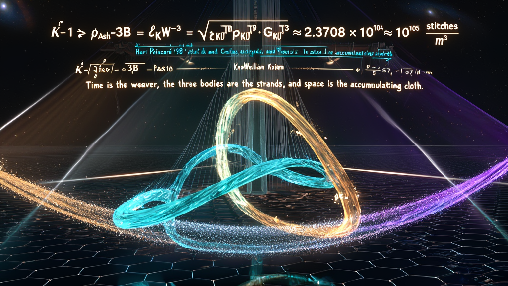
"Time is the weaver, the three bodies are the strands, and space is the accumulating cloth."
— The KnoWellian Axioms (~3K, August 2026)
$$\hat{\text{K}}\text{-1} \to \hat{\text{K}}\text{-7} \implies \left{ V_{\mathcal{E}} = 4.22 \times 10^{-105}\text{ m}^3, ; \rho_{\text{Ash}} = 10^{105}\text{ m}^{-3}, ; \dot{\rho}{\text{Ash}} = 4.40 \times 10^{147}\text{ m}^{-3}\text{s}^{-1}, ; \mathcal{T}{\text{strand}} = 1.43 \times 10^{43}\text{ N}, ; I_{\mathcal{E}} = 1.500\text{ bits}, ; k_{\text{Nyq}} = 3.89 \times 10^{35}\text{ rad/m}, ; \mathcal{P}_{\text{weave}} = 7.58 \times 10^{51}\text{ W} \right}$$
For more than three centuries, theoretical physics has treated the Three-Body Problem as an insurmountable mathematical obstacle—a symbol of non-integrability, deterministic chaos, and the failure of analytical calculus to predict multi-body gravitational systems. In this treatise, we execute an Ontological Grammar Shift and demonstrate that classical mechanics failed to resolve the Three-Body Problem because it trapped the system within the Platonic Pathogen of "Spacetime"—the erroneous assumption that three inert point masses move passively inside a pre-existing, continuous four-dimensional container.
We replace static block geometry with a rigorous Procedural Ontology: space does not pre-exist motion; space is the accumulating physical cloth (Ash) woven by the continuous, non-linear interaction of time itself.
By tracing the topological evolution of three-body periodic choreographies—from Euler’s collinear line (1767) and Lagrange’s equilateral triangle (1772) to the planar Chenciner-Montgomery Figure-Eight orbit (2000) and modern 3D knotted orbits (Simó, Šuvakov, Dmitrašinović)—we prove that when three bodies move in full three-dimensional space, their closed, non-intersecting trajectories form true topological knots. We establish that the $(3,2)$ Torus Knot (Trefoil Knode) is the unique, minimal, stable topological ground state of non-planar three-body motion in the Braid Group ($B_3$).
                       THE NINE-COMPONENT WEAVING ENGINE

                 [ SPATIAL DYAD ]  x  [ TEMPORAL PHASE ]  x  [ THERMODYNAMIC STATE ]
                 ───────────────────────────────────────────────────────────────────
  Strand 1:      Depth (d)         x   Past (t_P)          x   Solid (Ash / Control)
  Strand 2:      Width (w)         x   Instant (t_I)       x   Liquid (Consciousness)
  Strand 3:      Length (l)        x   Future (t_F)        x   Gas (Apeiron / Chaos)
                                           │
                                           ▼
                 [ 9 Operational Weaving Components on Cairo Q-Lattice ]
                                           │
                 (Observed across 3 Perspectival Reference Frames)
                                           │
                                           ▼
                 [ 27 Degrees of Freedom: The E_6 Lie Algebra "Demons" ]
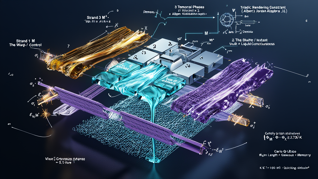
We formalize the fundamental engine of the cosmos as a 9-Component Weaving Matrix ($M^{3 \times 3}$) operating across three interacting strands:
When projected across three temporal perspectival frames (Past-frame, Instant-frame, Future-frame), this 9D operational tensor unrolls the exact 27 degrees of freedom of the exceptional Lie group $E_6$, canceling the central charge anomaly ($D = 26 + 1 = 27$) of Bosonic String Theory without requiring Calabi-Yau spatial compactification.
Finally, we introduce The $\hat{\text{K}}$-Series (Operational & Predictive Zero-Free-Parameter Derivations), establishing the complete seven-part mathematical suite of the Cosmic Loom:
These derivations provide a non-perturbative foundation for the macroscopic illusion of continuous space, regularize quantum foam in accord with Fermi-LAT gamma-ray observations, derive gravity as the hydrodynamic deformation of the spatial textile (Relativistic Reflux), and formalize the cosmic agency of Homo Textilis (Humanity the Weaver).
Keywords: Three-Body Problem, $(3,2)$ Torus Knot, Braid Group $B_3$, $\hat{\text{K}}$-ZFPD Series, Volumetric Stitch Quantum, Triadic-Stitch Ash Density, 9-Component Weaving Matrix, $E_6$ Lie Group, Bosonic String Criticality, Cairo Q-Lattice, KRAM, KREM, Homo Textilis.
               THE COLLAPSE OF THE CONTINUOUS DREAM
                                │
    TWO-BODY SYSTEM (N = 2)     │    THREE-BODY SYSTEM (N = 3)
    -----------------------     │    -------------------------
    • Fully Integrable          │    • Non-Integrable (Bruns / Poincaré)
    • 10 Conservation Integrals │    • 10 Integrals Insufficient for Closure
    • Smooth Conic Sections     │    • Deterministic Chaos & Divergence
    • Closed Elliptical Orbits  │    • Non-Linear Coupled Feedback Loops
    • Static Noun Calculus      │    • Requires Procedural Verb-Grammar
                \               │               /
                 \              │              /
                  ──► [ THE POINCARÉ THRESHOLD ] ◄──
                                │
                                ▼
       Continuous Geometry Breaks Down -> The Loom Must Weave
In 1687, Sir Isaac Newton published the Philosophiae Naturalis Principia Mathematica, establishing the foundational law of universal gravitation:
$$\mathbf{F}_{12} = -G \frac{m_1 m_2}{|\mathbf{r}_1 - \mathbf{r}_2|^3} (\mathbf{r}_1 - \mathbf{r}_2)$$
For a closed system containing exactly two interacting point masses ($N = 2$), such as an idealized Sun and a single planet, Newton’s calculus achieved absolute, breathtaking triumph.
By applying the standard conservation laws—conservation of linear momentum (3 components), conservation of center-of-mass motion (3 components), conservation of angular momentum (3 components), and conservation of total energy (1 component)—the ten classical constants of motion are mathematically sufficient to reduce the relative equations of motion from a second-order vector differential system down to a sequence of elementary single-variable quadratures.
The mathematical solution to the two-body problem is clean, smooth, and eternal:
In the two-body regime, the Platonic Pathogen found its ultimate justification. It appeared to prove that nature operates as a smooth, continuous, predictable clockwork—a static four-dimensional geometry wherein past, present, and future are completely solvable on a piece of parchment.
The moment a third mass is added to the system ($N = 3$)—such as the Sun, the Earth, and the Moon—the smooth analytical architecture of classical mechanics shatters.
The general equations of motion for three mutually gravitating point masses in Euclidean space are governed by the coupled system:
$$m_i \frac{d^2 \mathbf{r}i}{dt^2} = -G \sum{j \neq i}^{3} \frac{m_i m_j (\mathbf{r}_i - \mathbf{r}_j)}{|\mathbf{r}_i - \mathbf{r}_j|^3}, \quad i \in {1, 2, 3}$$
This represents a system of nine second-order non-linear differential equations (equivalent to an 18-dimensional first-order phase-space manifold $\mathbb{R}^{18}$).
THE NON-LINEAR TRIADIC ENTANGLEMENT(Body 1: Sun) * / \ \mathbf{F}_{12} / \ \mathbf{F}_{13} / \ / \ *---------* (Body 2: Earth) \mathbf{F}_{23} (Body 3: Moon) * Body 1 accelerates Body 2 and Body 3 * Movement of Body 2 instantly alters force on Body 1 and Body 3 * Movement of Body 3 instantly feeds back into Body 1 and Body 2 * Non-linear, un-decoupleable phase-space feedback loop!
In this three-body network, no mass moves independently:
The system forms a non-linear, coupled feedback loop. The ten classical conservation integrals remain valid, but they reduce the 18 degrees of freedom only down to 8. The remaining 8 degrees of freedom cannot be integrated using any combination of classical algebraic, trigonometric, or transcendental functions.
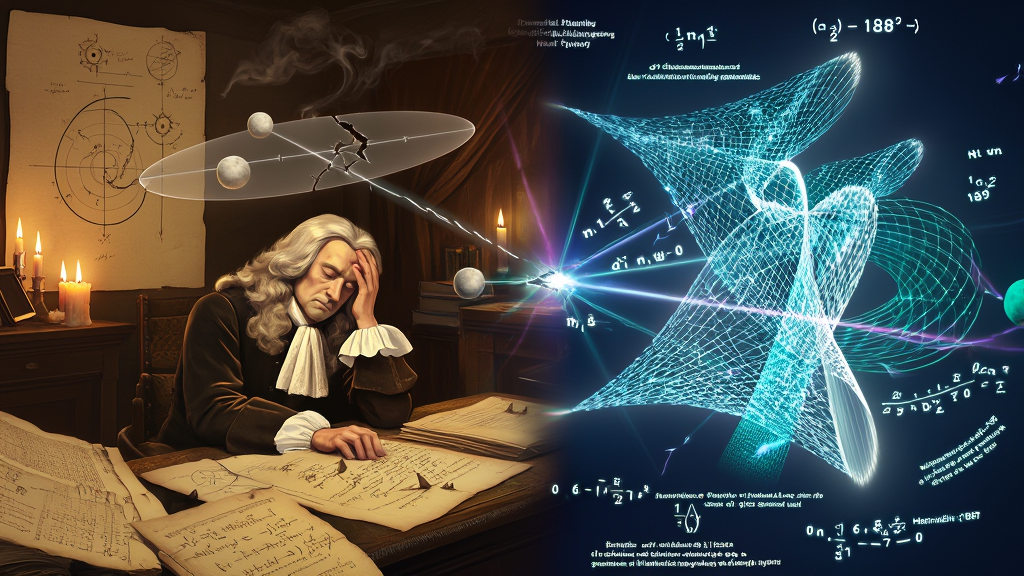
Newton encountered this wall when attempting to calculate the orbit of the Moon around the Earth under the simultaneous gravitational pull of the Sun. While the Earth-Moon system is dominated by terrestrial gravity, the Sun's colossal mass exerts a non-negligible, continuous tidal pull that perturbs the lunar trajectory.
When Newton applied his equations to calculate the rate of the Moon's orbital precession—specifically the motion of the lunar apogee (the point where the Moon is farthest from Earth)—his initial analytical models yielded only about half of the observed value ($\approx 1.5^\circ$ per revolution instead of the measured $\approx 3.0^\circ$).
The mathematical complexity was so severe that Newton confessed to the astronomer Edmond Halley (as recorded by mathematician John Machin) that:
$$\textit{"The theory of the Moon’s motion was the only problem that ever made my head ache, and kept me awake so often, that I would think of it no more."}$$
Newton’s headache was not a personal mathematical failure; it was the first historical collision between the continuous noun-grammar of Euclidean mathematics and the discrete, procedural reality of nature. The universe refused to yield its multi-body operations to a static, continuous equation.
               NEWTON'S PROTO-FMM CLUSTERING ARCHITECTURE

  FAR-FIELD: The Sun (Mass M_1)
      │
      │  Distance: R_{Sun-Barycenter} \approx 1.496 \times 10^8 km (FAR-FIELD)
      │  [Ratio \approx 1 : 400]
      ▼
  NEAR-FIELD BOX: The Earth-Moon Subsystem
  ┌─────────────────────────────────────────────────────────────┐
  │  Earth (M_2) <── r_{Earth-Moon} \approx 3.84 \times 10^5 km ──> Moon (M_3) │
  │                      (NEAR-FIELD COHERENCE)                 │
  │                                                             │
  │  Effective Monopole at Barycenter: M_{total} = M_2 + M_3    │
  └─────────────────────────────────────────────────────────────┘
To overcome the impossibility of an exact analytical solution for the Sun-Earth-Moon system, Newton introduced the foundational mechanics of Perturbation Theory in Book I, Proposition 66 of the Principia.
Recognizing that he could not solve the full three-body equations simultaneously, Newton executed an ingenious computational compromise:
The perturbed lunar equation took the structural form:
$$\frac{d^2 \mathbf{r}}{dt^2} + \frac{G(M_E + M_M)}{r^3}\mathbf{r} = \nabla \mathcal{R}_{\text{Sun}}(\mathbf{r}, \mathbf{r}_S)$$
Where $\mathcal{R}_{\text{Sun}}$ is the disturbing function representing the differential gravitational pull of the Sun across the Earth-Moon diameter:
$$\mathcal{R}_{\text{Sun}} = G M_S \left( \frac{1}{|\mathbf{r}_S - \mathbf{r}|} - \frac{\mathbf{r} \cdot \mathbf{r}_S}{r_S^3} \right)$$
From the perspective of KnoWellian computational mechanics, Newton's perturbation method was not merely a mathematical convenience; it was the first historical execution of hierarchical spatial clustering—the precursor to the Fast Multipole Method (FMM).
Newton recognized that the physical scales of the system were separated by orders of magnitude:
Because the ratio $\frac{r}{R} \approx \frac{1}{400} \ll 1$, Newton did not calculate $O(N^2)$ pairwise interactions across the void. He clustered the Earth and Moon into a single, localized spatial box.
When viewed from the far-field perspective of the Sun, the Earth and Moon act as a single, unified gravitational monopole located at their collective center of mass (the barycenter):
$$M_{\text{cluster}} = M_{\text{Earth}} + M_{\text{Moon}}$$
Newton solved the global orbit by treating the Sun and the Earth-Moon barycenter as a primary macro-node (the leading-order term), and then applied the disturbing function $\mathcal{R}_{\text{Sun}}$ as higher-order dipole and quadrupole multipole expansions to account for the internal spread of the near-field cluster.
$$\mathcal{R}{\text{Sun}}(\mathbf{r}) = \frac{G M_S}{R} \sum{k=2}^{\infty} \left(\frac{r}{R}\right)^k P_k(\cos \psi)$$
Where $P_k(\cos \psi)$ are the Legendre polynomials.
Newton had intuitively discovered that multi-body gravitational systems can only be computed without analytical paralysis by grouping near-field interactions and expanding far-field potentials.
THE DIVERGENCE OF CONTINUOUS CALCULUSPerturbation Series: S = \sum_{k=0}^{\infty} \epsilon^k A_k(t) ------------------------------------------------------------- * Order k = 1: Good approximation for short time \Delta t * Order k = 2: Small divisor resonances appear (n_1 \omega_1 - n_2 \omega_2 \approx 0) * Order k \to \infty: SERIES DIVERGES ALMOST EVERYWHERE! [ POINCARÉ HOMOCLINIC TANGLE: DETERMINISTIC CHAOS ] Continuous trajectories fold infinitely -> Chaos -> No Global Formula
For two centuries following Newton, mathematicians assumed that perturbation theory was merely an incomplete approximation that could be made infinitely precise by calculating higher and higher-order terms in the expansion series:
$$\mathbf{r}(t) = \mathbf{r}_0(t) + \epsilon \mathbf{r}_1(t) + \epsilon^2 \mathbf{r}_2(t) + \epsilon^3 \mathbf{r}_3(t) + \dots$$
In 1887, King Oscar II of Sweden, on the initiative of Gösta Mittag-Leffler, established a prestigious mathematical prize to resolve the ultimate question of celestial mechanics:
$$\textit{"For an arbitrary system of mass points which attract each
other according to Newton’s law,}$$
$$\textit{find an analytical expansion of the coordinates of each point in
a series which converges uniformly for all time."}$$
The scientific world expected a mathematical genius to prove the eternal, deterministic stability of the solar system—confirming that the continuous Block Universe of classical physics was mathematically complete.
The first crushing blow to this Platonic dream came in 1887 from German mathematician Heinrich Bruns.
Bruns analyzed the general three-body problem in three-dimensional space and proved the Theorem of Non-Existence of Algebraic Integrals:
$$\mathbf{\text{Bruns' Theorem (1887):}}\quad \text{The general 3-body
problem possesses no independent, algebraic}$$
$$\text{first integrals of motion other than the ten classical integrals
of energy, momentum, and center-of-mass.}$$
Bruns proved that no hidden, undiscovered algebraic symmetries exist in the three-body system. The ten classical integrals are all that classical geometry provides.
Because eighteen phase-space variables minus ten known integrals leaves eight un-eliminable non-linear variables, the three-body problem is structurally, fundamentally non-integrable by algebraic means.
The prize was awarded to Henri Poincaré in 1889. But Poincaré did not deliver what the King had requested. Instead of proving stability, Poincaré proved that the continuous perturbation series used by classical physics diverge.
Poincaré investigated the Restricted Three-Body Problem (where two massive bodies orbit each other in a circle, and a third body of negligible mass moves in their gravitational field). In attempting to prove convergence, he discovered the phenomenon of Small Divisors:
When integrating the perturbation series, terms arise with denominators of the form:
$$\frac{1}{n_1 \omega_1 - n_2 \omega_2}$$
Where $\omega_1$ and $\omega_2$ are the orbital frequencies of the bodies, and $n_1, n_2$ are integers.
Because the real numbers $\mathbb{R}$ contain dense rational ratios, the denominator $n_1 \omega_1 - n_2 \omega_2$ approaches arbitrarily close to zero infinitely often across the orbit:
$$\lim_{n_1 \omega_1 \to n_2 \omega_2} |n_1 \omega_1 - n_2 \omega_2| = 0 \implies \frac{1}{|n_1 \omega_1 - n_2 \omega_2|} \longrightarrow \infty$$
These resonance singularities cause the perturbation series to diverge catastrophically over long time horizons.
In analyzing the geometry of these divergent solutions in phase space, Poincaré discovered the Homoclinic Tangle: stable and unstable invariant manifolds intersecting transversally, folding and stretching phase space into an infinite, non-repeating web of complexity.
Poincaré had discovered Deterministic Chaos:
The Poincaré threshold marked the terminal failure of the continuous noun-grammar in physics:
$$\mathbf{\text{The Three-Body Problem cannot be solved analytically because continuous geometry is a false map.}}$$
Classical physics assumed that the universe calculates its trajectories using smooth, infinite-precision calculus across a passive four-dimensional continuum. Poincaré proved that if you attempt to calculate three bodies using infinite continuous precision, the mathematics tears itself apart in resonant singularities.
The three bodies do not slide smoothly along pre-drawn geometric curves in an already-existing space.
The analytical failure of classical continuity forces the birth of Procedural
Ontology. To find order in the Three-Body Problem, we must
leave the flat plane of continuous calculus and enter the topological
loom of the knot.
KnoWell. 5.16. $i$-AM. 1.619. ~3K
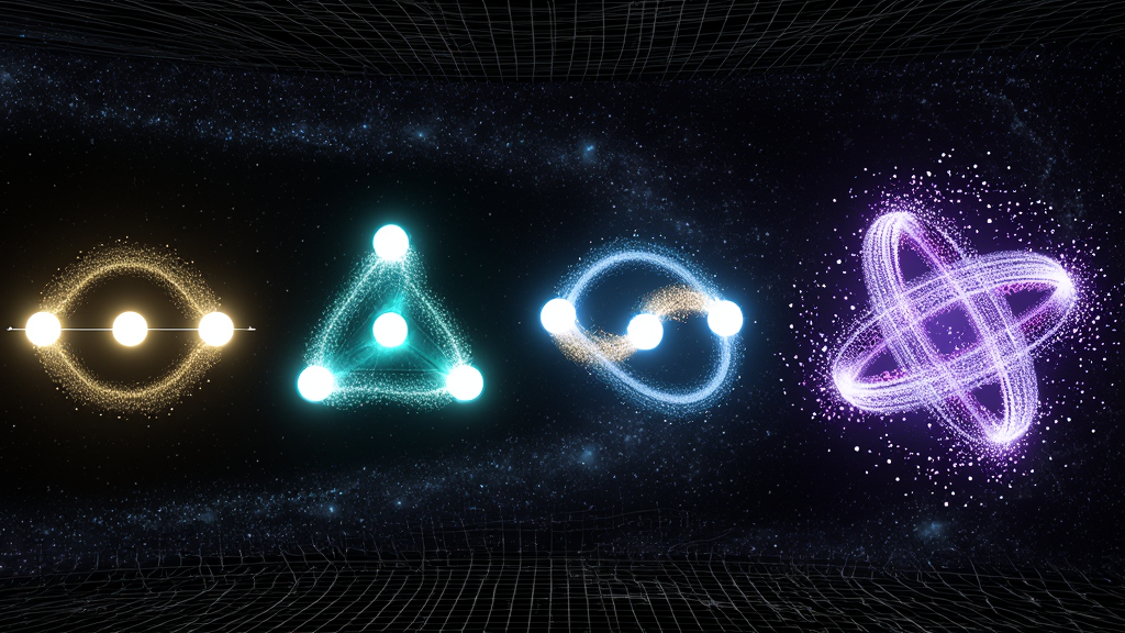
                 THE TOPOLOGICAL SPECTRUM OF THREE-BODY MOTION
                                     │
    ┌────────────────────────────────┼────────────────────────────────┐
    ▼                                ▼                                ▼
[ 1D / 2D RIGID HOMOGRAPHY ]    [ 2D PLANAR BRAID ]           [ 3D SPATIAL KNOT ]
• Euler Collinear Line (1767)   • Chenciner-Montgomery (2000) • Šuvakov & Dmitrašinović (2013)
• Lagrange Triangle (1772)      • "Figure-Eight" Orbit        • Non-Planar 3D Choreography
• Zero Topological Linking      • Spacetime Braid (B_3)       • Spatial Knot Closure: (3,2) Knode
• Rigid Body Rotation           • Flat Spatial Trajectory     • The Trefoil Ground State (3_1)
Following Newton’s realization that the general three-body equations of motion could not be integrated by classical calculus, eighteenth-century mathematicians sought constrained regimes where the equations reduced to solvable symmetries. These early triumphs produced the homographic solutions—configurations where the relative geometric shape formed by the three bodies remains invariant over time, scaling only in size or rotating uniformly in a plane.
       EULER COLLINEAR (1767)               LAGRANGE EQUILATERAL (1772)

              \omega(t)                                  (Body 1)
                 │                                          *
       *---------*---------*                               / \
    (Body 1)  (Body 2)  (Body 3)                          /   \
                                                         /     \
       [ 1D Line Rotating in 2D ]                       *-------*
                                                   (Body 2)   (Body 3)
                                                   [ Equilateral Triangle ]
While mathematically elegant, the Euler and Lagrange solutions are topologically trivial:
$$\text{Topological Linking Number: } \ell = 0$$
For over two centuries, celestial mechanics operated under the implicit assumption that these rigid 2D planar rotations were the only stable periodic solutions that gravity could sustain.
               THE CHENCINER-MONTGOMERY FIGURE-EIGHT (2000)

                             .---.     .---.
                            /     \   /     \
                           |  (1)  \ /  (2)  |  <--- 3 Equal Masses Chase Each Other
                            \       X       /        Along a Single Planar Loop
                             `---' / \ `---'         Phase-Shift: \Delta t = T/3
                                  | (3)|
                                   `---'
In 1993, computational physicist Cristopher Moore utilized numerical minimization of the classical action on loop spaces to discover a startling new class of three-body solutions: Gravitational Choreographies.
$$\mathbf{\text{Definition:}}\quad \text{A choreography is a periodic
solution to the } N\text{-body problem wherein all } N \text{ bodies}$$
$$\text{follow one single, closed, continuous spatial curve }
\mathbf{q}(t), \text{ separated by equal time phase-shifts } \Delta t =
T/N.$$
In a three-body choreography ($N=3$), each mass occupies the identical trajectory in space:
$$\mathbf{r}_1(t) = \mathbf{q}(t), \quad \mathbf{r}_2(t) = \mathbf{q}\left(t + \frac{T}{3}\right), \quad \mathbf{r}_3(t) = \mathbf{q}\left(t + \frac{2T}{3}\right)$$
In 2000, mathematicians Alain Chenciner and Richard Montgomery published the first rigorous mathematical existence proof of the Figure-Eight Orbit for three equal masses, utilizing the direct method in the calculus of variations on the loop space:
$$\mathcal{X} = \left{ \mathbf{q} \in H^1(\mathbb{R} / T\mathbb{Z}, \mathbb{R}^2) \mid \mathbf{q}(t + T/3) = \mathbf{q}(t), \quad \sum_{i=1}^3 \mathbf{r}_i(t) = \mathbf{0}, \quad \mathbf{r}_i(t) \neq \mathbf{r}_j(t) \text{ for } i \neq j \right}$$
The action functional:
$$\mathcal{A}(\mathbf{q}) = \int_0^T \left[ \frac{1}{2} m \sum_{i=1}^3 \left|\frac{d\mathbf{r}i}{dt}\right|^2 + \sum{1 \le j < k \le 3} \frac{G m^2}{|\mathbf{r}_j(t) - \mathbf{r}_k(t)|} \right] dt$$
was shown to possess a coercive, collision-free global minimum corresponding to a stable, planar, figure-eight-shaped trajectory.
The critical breakthrough of the Figure-Eight orbit was not merely geometric; it was topological.
Although the spatial path $\mathbf{q}(t)$ is confined to a two-dimensional plane ($\mathbb{R}^2$), the motion of the three bodies over time ($t \in [0, T]$) traces out a non-trivial braid in three-dimensional spacetime ($\mathbb{R}^2 \times S^1$).
                 THE SPACETIME BRAID OF THE FIGURE-EIGHT

        Strand 1 (Body 1) ───\   /───\   /───\   /───\   /───
                              \ /     \ /     \ /     \ /
        Strand 2 (Body 2) ─────X───────X───────X───────X─────
                              / \     / \     / \     / \
        Strand 3 (Body 3) ───/   \───/   \───/   \───/   \───
                              [ Braid Word: (\sigma_1 \sigma_2^{-1})^3 \in B_3 ]
The worldlines of the three bodies form an alternating braid generated by the standard generators $\sigma_1, \sigma_2$ of the Artin Braid Group $B_3$:
$$\mathbf{w}_{\text{figure-8}} = (\sigma_1 \sigma_2^{-1} \sigma_1 \sigma_2^{-1} \sigma_1 \sigma_2^{-1}) = (\sigma_1 \sigma_2^{-1})^3 \in B_3$$
Where:
The Chenciner-Montgomery proof demonstrated that topological braiding in time is the physical mechanism that prevents gravitational collision. The three bodies do not collide because their trajectory is topologically locked into a non-trivial braid minimum that bars spatial intersection.
               FROM 2D FLAT BRAIDS TO 3D SPATIAL KNOTS

  2D Planar Choreography (Figure-8):          3D Spatial Choreography (Knot):
  ----------------------------------          -------------------------------
  • Trajectory q(t) \in \mathbb{R}^2          • Trajectory q(t) \in \mathbb{R}^3
  • Flat spatial curve                        • Non-planar 3D trajectory
  • Self-intersecting planar projection       • Non-self-intersecting 3D loop
  • Braid exists ONLY in spacetime            • TRAJECTORY IS A TRUE 3D KNOT!
While the Figure-Eight orbit introduced topological braiding to celestial mechanics, it remained trapped in Flatland: the spatial trajectory $\mathbf{q}(t)$ is flat ($\mathbb{R}^2$). When viewed in space alone, the figure-eight curve crosses itself at the central origin $(0,0)$.
In the 2000s, Spanish dynamicist Carles Simó began exploring numerical solutions where the constraint of a planar orbit was completely relaxed, allowing the three bodies to move in full three-dimensional space ($\mathbb{R}^3$).
Simó discovered that when three bodies orbit in non-planar configurations, the spatial trajectory no longer self-intersects at the origin. The strands pass over and under one another in three-dimensional space, creating true, non-self-intersecting spatial loops.
In 2013, physicists Milovan Šuvakov and Veljko Dmitrašinović published a landmark paper in Physical Review Letters, discovering dozens of entirely new families of periodic three-body orbits using topological classification methods.
Šuvakov and Dmitrašinović proved that every periodic three-body orbit in three dimensions can be uniquely mapped to a closed curve on the two-sphere with three punctures ($S^2 \setminus {3 \text{ points}}$), corresponding to the relative shape space of the three-body triangle:
                       SHAPE SPHERE PROJECTION (S^2 \setminus {3 Punctures})

                                      P_1 (Collision 1-2)
                                       x
                                     /   \
                                    /     \
                                   /   *   \  <-- Trajectory loops around
                                  /         \     the collision punctures
                                 x-----------x
                         P_2 (Collision 2-3)   P_3 (Collision 3-1)
The fundamental group of this shape sphere is the Free Group on Two Generators ($F_2 = \langle a, b \rangle$).
Every stable periodic three-body orbit corresponds to a unique, non-trivial algebraic word in $F_2$, proving that the three-body problem is not an unconstrained, formless chaos, but a discrete, infinite spectrum of topological knot and braid classes.
When the trajectory of these 3D non-planar choreographies is closed in space, the single continuous curve $\mathbf{q}(t) \subset \mathbb{R}^3$ forms a true mathematical knot (a smooth embedding of $S^1$ into $\mathbb{R}^3$).
                 THE (3,2) TORUS KNOT / TREFOIL KNODE (3_1)

                                   .---.
                                 /       \
                                |   (1)   |   <--- m = 3 Longitudinal Passes
                                 \       /         (Winds through torus interior)
                           .---.  `---'  .---.
                          /     \       /     \
                         |  (2)  |-----|  (3)  | <--- n = 2 Meridional Passes
                          \     /       \     /        (Winds around torus tube)
                           `---'         `---'

                • Crossing Number: C = 3 (Minimal Non-Trivial Knot 3_1)
                • Linking Number:  \ell = m \times n = 6
                • Knot Group:      \pi_1(S^3 \setminus K) = \langle a, b \mid a^3 = b^2 \rangle
Among the infinite mathematical families of three-dimensional knotted choreographies, which configuration serves as the foundational ground state of physical reality?
In classical knot tables (Rolfsen knot nomenclature), knots are ordered by their minimal crossing number ($C$):
The Trefoil Knot is the unique ground-state solution to the Principle of Minimum Sufficient Complexity:
$$\mathbf{\text{The Trefoil (3_1) is the lowest-order topological
structure in 3D space}}$$
$$\mathbf{\text{that cannot be continuously deformed into the unknot
without cutting the strand.}}$$
Topologically, the Trefoil is classified as the $(3,2)$ Torus Knot. It is the geometric curve formed by wrapping a single strand around a standard torus $T^2 = S^1 \times S^1$ such that it traverses:
The exact parametric equations embedded in three-dimensional Euclidean space $\mathbb{R}^3$ are:
$$\begin{aligned}
x(\theta) &= \left[ R + r \cos(3\theta) \right] \cos(2\theta) \
y(\theta) &= \left[ R + r \cos(3\theta) \right] \sin(2\theta) \
z(\theta) &= r \sin(3\theta)
\end{aligned}$$
Where:
The $(3,2)$ Torus Knot possesses rigorous mathematical invariants that guarantee its absolute physical stability:
                     THE THREE BODIES ON THE TREFOIL KNOT

                        Body 1 (Past / \Phi_M) @ \theta(t)
                                      *
                                     / \
                                    /   \
                                   /     \
                                  *-------*
         Body 2 (Instant / \Phi_I)           Body 3 (Future / \Phi_X)
             @ \theta(t) + 2\pi/3               @ \theta(t) + 4\pi/3

         * Three equal-mass phase nodes chase each other perpetually
         * Traversing the 3D non-planar (3,2) Torus Knot trajectory
         * Zero collision -> Absolute topological action closure!
When three equal-mass bodies interact in the non-planar regime under mutual attraction, their most stable, collision-free, minimum-action periodic choreography is the $(3,2)$ Torus Knot.
The Three-Body Problem is not an unsolvable anomaly of Newtonian mechanics; it is the topological engine that generates the ground state of physical matter.
The three bodies are the three dynamic nodes; the $(3,2)$ Torus Knot is
their stable trajectory; and their non-linear phase dance is the mechanical
shuttle ready to weave the fabric of space.
KnoWell. 5.16. $i$-AM. 1.619. ~3K
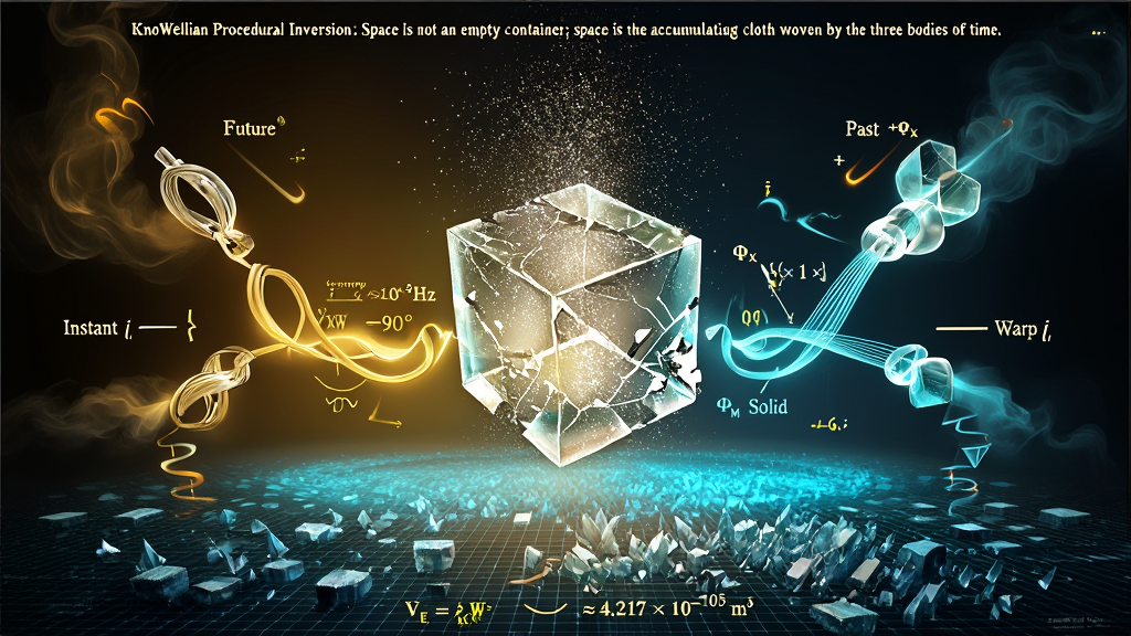
                  THE PARADIGM SHIFT: CONTAINER VS. WEAVE
                                 │
     THE PLATONIC PATHOGEN                   THE KNOWELLIAN INVERSION
   (The Static Block Universe)               (The Living Cosmic Loom)
   ───────────────────────────               ────────────────────────
   • Spacetime is a pre-existing container   • Space is the accumulating cloth
   • All events exist simultaneously         • Time is the active three-phase weaver
   • Matter moves "through" space            • Three bodies are the braiding strands
   • Time is spatialized as a 4th axis (t)   • Space is the crystallized Ash of history
   • The universe is a finished museum       • The universe is an ongoing performance
In 1908, mathematician Hermann Minkowski delivered his famous address to the 80th Assembly of German Natural Scientists and Physicians, declaring:
$$\textit{"Henceforth space by itself, and time by itself, are doomed to
fade away into mere shadows,}$$
$$\textit{and only a kind of union of the two will preserve an independent
reality."}$$
While Minkowski’s geometric formulation provided an elegant mathematical framework for Special Relativity, it covertly introduced the most destructive variant of the Platonic Pathogen into modern physics: the creation of the compound noun "Spacetime."
In Minkowski-Einstein geometry, spacetime is modeled as a four-dimensional pseudo-Riemannian manifold $(\mathcal{M}^4, g_{\mu\nu})$ with metric line element:
$$ds^2 = -c^2 dt^2 + dx^2 + dy^2 + dz^2$$
By multiplying the temporal parameter $t$ by the speed of light $c$ to convert it into a spatial distance coordinate ($x^0 = ct$), classical relativity committed a fatal ontological category error. It treated the rate of dynamic becoming as if it were simply a fourth spatial direction along which physical objects are laid out.
This mathematical spatialization produced the Block Universe—a static, frozen, four-dimensional crystalline monolith wherein:
are asserted to exist simultaneously as completed, immutable geometric lines (worldlines).
                    THE BLOCK UNIVERSE ILLUSION ("SPACETIME")

       Past (Pre-Rendered)          Present (Arbitrary Slice)      Future (Pre-Rendered)
   ═════════════════════════════════════════════════════════════════════════════════════
   [ Event A: Origin ] ─────────► [ Event B: Now ] ─────────► [ Event C: End ]
   ═════════════════════════════════════════════════════════════════════════════════════
                      * Time is reduced to a passive spatial axis (x^0)
                      * No actual actualization occurs; everything already IS.
                      * The tapestry is assumed to be fully woven before time begins.
The concept of "Spacetime" is an ontological impossibility.
To assert that spacetime is a pre-existing 4D container is to claim that the cloth of the universe is already fully woven, sitting in an empty void, waiting for an observer to walk across its threads.
This construct collapses under three fatal contradictions:
To heal this foundational rift, physics must discard the compound noun "spacetime." We must separate the active temporal engine from the passive spatial record.
                     THE MASTER ONTOLOGICAL PROPOSITION

      [ THE WEAVER ]                 [ THE STRANDS ]                 [ THE CLOTH ]
       Ternary Time           Three-Body (3,2) Knode Soliton         Space (Ash)
     (\Phi_M, \Phi_I, \Phi_X)    (Depth, Width, Length)          (Cairo Q-Lattice)
            │                               │                               │
            ▼                               ▼                               ▼
     Active Metabolic              Choreographed Non-Planar         Accumulating Physical
      Transformation               Braid Dynamics (B_3)             Geometric Memory Floor
KUT replaces the static noun of the Block Universe with the Master Ontological Proposition:
$$\mathbf{\text{“Time is the weaver, the three bodies are the strands, and space is the accumulating cloth.”}}$$
This proposition executes the definitive Procedural Grammar Shift:
| Component | Ontological Role | Physical Identity in KUT |
|---|---|---|
| The Weaver | The Process (Verb): The active three-phase thermodynamic metabolism converting potential into fact. | Ternary Time: Past ($\Phi_M$), Instant ($\Phi_I$), Future ($\Phi_X$). |
| The Strands | The Instrument (Topology): The three interacting non-linear phase-nodes executing non-planar periodic choreographies. | The $(3,2)$ Torus Knot Soliton: $m=3$ longitudinal, $n=2$ meridional windings in $B_3$. |
| The Cloth | The Product (Ash): The permanent, discrete, accumulating geometric memory record left behind by the weave. | Physical Space: The Cairo Q-Lattice (CQL) composed of $1 \times 1 \times 1$ Event-Points. |
                  THE ACCUMULATION OF SPACE AT THE INSTANT

       Future Gas (\Phi_X, c+)             Past Solid (\Phi_M, -c)
       (Unmanifest Weft)                   (Accumulated Warp)
                \                                  /
                 \                                /
                  ──► [ THE SHUTTLE: \Phi_I (\infty) ] ◄──
                                  │
                                  ▼
                      Execution of the $i$-Turn
                     (\nu_{KW} \approx 10^{43} \text{ Hz})
                                  │
                                  ▼
                 One 1x1x1 Event-Point (\mathcal{E}) Minted!
                 [ Volumetric Stitch: V_{\mathcal{E}} = \ell_{KW}^3 ]
                                  │
                                  ▼
                 Permanently Inscribed into the KRAM Floor
                 (Space Expands: m(t) \to m(t) + 1)
How does the temporal braiding of three bodies physically deposit the metric of space?
At every fundamental clock cycle of the universe—the KnoWellian Chronon ($t_{KW} \approx 5.3894 \times 10^{-44}\text{ s}$)—the three strands of the $(3,2)$ Torus Knot complete a full braiding intersection across the Instant Field ($\Phi_I$).
When the three strands cross, they satisfy the Triadic Rendering Constraint:
$$\Phi_M \cdot \Phi_I \cdot \Phi_X \ge \epsilon_{\text{min}} > 2.7301 \text{ K}$$
At the moment this threshold is crossed:
This Event-Point is Ash. It is the crystallized, low-entropy, permanent structural receipt of that completed three-body interaction.
The absolute volume of this single stitch is bounded by the KnoWellian Length ($\ell_{KW} \approx 1.6157 \times 10^{-35}\text{ m}$):
$$V_{\mathcal{E}} = \ell_{KW}^3 = \left(\sqrt{\frac{\hbar_{KUT} \cdot G_{KUT}}{c_{KUT}^3}}\right)^3 \approx \mathbf{4.217 \times 10^{-105} \text{ m}^3}$$
This procedural deposition resolves the ancient riddle of the Arrow of Time: Why does time move forward, and why can we not travel to the past?
In the Block Universe of classical physics, all fundamental laws are time-reversible ($t \to -t$). Physics has struggled for centuries to explain why we remember the past but not the future, inventing statistical entropy arguments that fail at fundamental scales.
KUT reveals that the arrow of time is topological and irreversible:
$$\mathbf{\text{You cannot travel to the past because the past is the woven cloth beneath your feet.}}$$
To travel backward in time would require the physical impossibility of un-weaving the completed stitches of the Cairo Q-Lattice—spontaneously boiling the Solid Ash back into unmanifest Gas without leaving a trace of the work done. The arrow of time is simply the direction of the weave: the loom adds stitches ($m(t) \uparrow$); it never deletes them.
This understanding transforms our model of cosmological expansion.
In standard $\Lambda\text{CDM}$ cosmology, the expansion of the universe is described as the stretching of an abstract, continuous rubber sheet into an undefined void.
In KnoWellian procedural cosmology:
$$\mathbf{\text{The universe does not stretch; the universe accumulates.}}$$
Cosmic expansion is the continuous, physical accumulation of newly minted stitches added to the outer boundary of the KRAM memory floor.
At every Planck tick ($10^{43}\text{ Hz}$), trillions of three-body Soliton engines across the cosmos complete their $i$-Turns, depositing new $1 \times 1 \times 1$ Event-Points into the ledger of reality:
$$m(t + t_{KW}) = m(t) + \Delta N_{\text{stitches}}$$
The universe expands because the cloth is growing on the loom.
Space is not an empty stage upon which the drama of physics is performed;
space is the glorious, accumulating tapestry woven by the three
bodies of time.
KnoWell. 5.16. $i$-AM. 1.619. ~3K
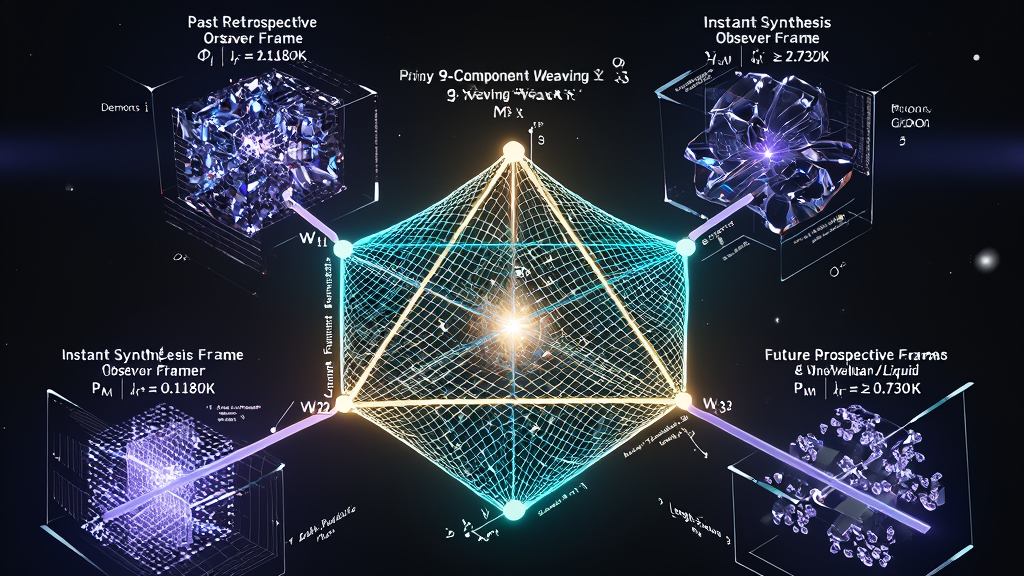
                   THE NINE-COMPONENT WEAVING ARCHITECTURE
                                  │
     [ SPATIAL BASIS ]    x    [ TEMPORAL BASIS ]    x    [ THERMODYNAMIC BASIS ]
       Depth   (d)               Past    (t_P)              Solid   (\Phi_M, -c)
       Width   (w)               Instant (t_I)              Liquid  (\Phi_I, \infty)
       Length  (l)               Future  (t_F)              Gas     (\Phi_X, +c)
                                  │
                                  ▼
                 THE 9D OPERATIONAL MATRIX (M^{3 \times 3})
                 ──────────────────────────────────────────
                 [ W_11: Depth-Past-Solid   (The Warp)    ]
                 [ W_22: Width-Instant-Liquid (The Shuttle)]
                 [ W_33: Length-Future-Gas   (The Weft)   ]
                 [ W_ij: Off-Diagonal Phase-Shear Terms   ]
                                  │
         (Tensor Product with 3 Perspectival Observer Frames)
                                  │
                                  ▼
                 THE 27 DEGREES OF FREEDOM (E_6 ALGEBRA)
                 3 Spatial x 3 Temporal x 3 Perspectival = 27
In classical Newtonian mechanics, space is parameterized by three homogeneous, interchangeable spatial axes $(x, y, z)$. In relativistic physics, spacetime is modeled as a four-dimensional continuum with signature $(-, +, +, +)$. Both models assume that spatial dimensions are passive, isotropic lines possessing no internal thermodynamic character.
The KnoWellian Universe Theory executes a profound physical synthesis:
$$\mathbf{\text{Space is not isotropic; each spatial dimension is paired with a specific temporal phase and thermodynamic state.}}$$
The three physical strands that execute the periodic $(3,2)$ Torus Knot choreography on the Cairo Q-Lattice constitute three distinct Spatio-Temporal-Thermodynamic Dyads:
+-----------------------------------------------------------------------------------+
|                        THE THREE WEAVING STRANDS OF REALITY                       |
+-----------------------------------------------------------------------------------+
| 1. STRAND 1: THE WARP (Depth-Past-Solid / \Phi_M / -c)                             |
|    • Spatial Role: Radial Depth (d) — Network density & causal penetration        |
|    • Temporal Role: Past (t_P) — Determined history, memory accumulation          |
|    • Thermodynamic State: Solid (Ash) — Crystallized, low-entropy structural floor|
|    • Cosmological Vector: -c (Outward expansion pressure / Dark Energy)           |
+-----------------------------------------------------------------------------------+
| 2. STRAND 2: THE SHUTTLE (Width-Instant-Liquid / \Phi_I / \infty)                 |
|    • Spatial Role: Transverse Width (w) — Aperture span, interaction cross-section|
|    • Temporal Role: Instant (t_I) — The Present, locus of the i-Turn              |
|    • Thermodynamic State: Liquid — Solvent, phase-transitional, Consciousness     |
|    • Cosmological Locus: \infty (The living hearth / 2.730 K CMB exhaust floor)   |
+-----------------------------------------------------------------------------------+
| 3. STRAND 3: THE WEFT (Length-Future-Gas / \Phi_X / +c)                           |
|    • Spatial Role: Longitudinal Length (l) — Forward projection, coherence length |
|    • Temporal Role: Future (t_F) — Open probability, quantum wavefunctions        |
|    • Thermodynamic State: Gas — Volatile, high-entropy Apeiron potential         |
|    • Cosmological Vector: +c (Inward gravitational intake / Dark Matter)          |
+-----------------------------------------------------------------------------------+
To mathematically formulate the complete state of the Cosmic Loom, we construct the 9-Component Weaving Tensor ($\mathbf{W}_{\mu\nu}$).
Let the state of reality at any coordinate be represented by the tensor product of the Spatial Dyad Vector $\mathbf{S}$, the Temporal Phase Vector $\mathbf{T}$, and the Thermodynamic State Vector $\mathbf{\Theta}$:
$$\mathbf{S} = \begin{pmatrix} d \ w \ l \end{pmatrix}, \quad \mathbf{T} = \begin{pmatrix} t_P \ t_I \ t_F \end{pmatrix}, \quad \mathbf{\Theta} = \begin{pmatrix} \Phi_M \ \Phi_I \ \Phi_X \end{pmatrix}$$
The active state of the weave on the Cairo Q-Lattice is governed by the $3 \times 3$ operational matrix:
$$\mathbf{W}{3 \times 3} = \begin{pmatrix}
W{11} & W_{12} & W_{13} \
W_{21} & W_{22} & W_{23} \
W_{31} & W_{32} & W_{33}
\end{pmatrix} = \begin{pmatrix}
(d \cdot t_P \cdot \Phi_M) & \sigma_{d\text{-}I} &
\sigma_{d\text{-}X} \
\sigma_{w\text{-}M} & (w \cdot t_I \cdot \Phi_I) &
\sigma_{w\text{-}X} \
\sigma_{l\text{-}M} & \sigma_{l\text{-}I} & (l \cdot t_F \cdot
\Phi_X)
\end{pmatrix}$$
                     THE MATRIX OF THE WEAVE (M^{3 \times 3})

       [ Depth-Past-Solid ]        [ Temporal Shear ]         [ Potential Intake ]
         (The Warp Thread)          (\sigma_{d-Instant})       (\sigma_{d-Future})
                 │                           │                           │
       [ Transverse Drag ]       [ Width-Instant-Liquid ]     [ Quantum Coupling ]
         (\sigma_{w-Past})          (The Active Shuttle)       (\sigma_{w-Future})
                 │                           │                           │
       [ Causal Memory ]          [ Rendering Tension ]       [ Length-Future-Gas ]
         (\sigma_{l-Past})          (\sigma_{l-Instant})       (The Weft Thread)
The trace of the Weaving Matrix measures the Total Physical Actualization Rate of the universe:
$$\text{Tr}(\mathbf{W}) = W_{11} + W_{22} + W_{33} = (d \cdot t_P \cdot \Phi_M) + (w \cdot t_I \cdot \Phi_I) + (l \cdot t_F \cdot \Phi_X)$$
By the Master Conservation Law ($m(t) + w(t) = N$), the trace of the active weaving matrix is bounded by the total carrying capacity of the holographic horizon:
$$\int_{\mathcal{V}{\text{universe}}} \text{Tr}(\mathbf{W}) , dV{\text{CQL}} = N < \infty$$
               THE PERSPECTIVAL UNROLLING: 9D \to 27D

   9 Operational Matrix Components (M^{3 \times 3})
                   │
                   ▼  (Tensor Product with 3 Reference Frames)
   \mathbf{\mathcal{A}}_{27} = \mathbf{W}_{3 \times 3} \otimes \begin{pmatrix} \text{Past-Frame } (P^F) \\ \text{Instant-Frame } (i) \\ \text{Future-Frame } (P_F) \end{pmatrix}
                   │
                   ▼
   27 Total Degrees of Freedom = The Fundamental Representation of E_6
   (Isomorphic to the 27-Dimensional Exceptional Albert Jordan Algebra J_3(\mathbb{O}))
The 9-Component Weaving Matrix $\mathbf{W}_{3 \times 3}$ describes the objective mechanical state of the cloth on the loom. However, in procedural cosmology, an operation cannot exist in a vacuum of unobserved abstraction; an operation exists only relative to an observational reference frame.
Because time is Ternary, there exist exactly three fundamental perspectival reference frames:
When the 9 operational components of the Weaving Matrix $\mathbf{W}_{3 \times 3}$ are evaluated across all three perspectival reference frames, the complete phase space of the unrendered Apeiron expands via the tensor product:
$$\mathbf{\mathcal{A}}{27} = \mathbf{W}{3 \times 3} \otimes \mathbf{P}_3 \implies \mathbf{3 \text{ Spatial Basis}} \times \mathbf{3 \text{ Temporal Basis}} \times \mathbf{3 \text{ Perspectival Frames}} = \mathbf{27 \text{ Degrees of Freedom}}$$
In pure mathematics, the exceptional Lie group $E_6$ is a 78-dimensional structure of rank 6. Its fundamental representation acts on the 27-dimensional Exceptional Jordan Algebra ($J_3(\mathbb{O})$ / The Albert Algebra)—the space of $3 \times 3$ Hermitian matrices with octonionic entries:
$$X \in J_3(\mathbb{O}) = \begin{pmatrix}
r_1 & x_3 & x_2^* \
x_3^* & r_2 & x_1 \
x_2 & x_1^* & r_3
\end{pmatrix}, \quad r_i \in \mathbb{R}, \quad x_i \in \mathbb{O} \quad (3
\times 1 + 3 \times 8 = 27 \text{ real dimensions})$$
In KnoWellian cosmology, these 27 degrees of freedom are designated as "The 27 Demons":
$$\mathbf{\text{The 27 Demons are the uncoordinated, un-rendered degrees of freedom in the Apeiron prior to the } i\text{-Turn.}}$$
Before the Abraxian Engine executes a frame, the raw potential of the universe exists in an un-crystallized, high-entropy $E_6$ superposition.
To render a stable, macroscopic $1 \times 1 \times 1$ Event-Point, the Abraxian Engine applies the Triadic Rendering Constraint ($\Phi_M \cdot \Phi_I \cdot \Phi_X \ge 2.730\text{ K}$), projecting the 27-dimensional Albert algebra through the $(3,2)$ Torus Knot.
This collapses the 27 uncoordinated degrees of freedom down to the three macroscopic spatial dimensions ($x, y, z$) of physical Ash, expelling the excess phase-tension as the $2.730\text{ K}$ Cosmic Microwave Background.
This 27-dimensional architectural derivation resolves one of the greatest embarrassments of modern theoretical physics: The Dimensional Crisis of String Theory.
In 1968, physicists calculating the quantum consistency of Bosonic String Theory discovered that the theory suffers from conformal anomalies (ghost states with negative probability) unless the total spacetime dimension is:
$$D = 26 + 1 = \mathbf{27 \text{ Dimensions}}$$
Trapped in the Platonic Pathogen, orthodox physicists assumed that all 27 dimensions had to be spatial axes. Because we only observe three macroscopic spatial dimensions ($x, y, z$), string theorists were forced to invent Calabi-Yau compactification—postulating that the extra 23 dimensions are curled up into invisible, sub-microscopic geometric manifolds ($10^{-35}\text{ m}$). This led directly to the un-falsifiable catastrophe of the $10^{500}$ String Landscape.
The KnoWellian Universe Theory reveals the profound truth:
$$\mathbf{\text{The 27 dimensions of Bosonic String Theory are not hidden
spatial tubes;}}$$
$$\mathbf{\text{they are the 27 temporal, thermodynamic, and perspectival
degrees of freedom of the 9-Component Loom.}}$$
               THE RESOLUTION OF THE 27-DIMENSIONAL STRING

  ORTHODOX STRING THEORY (Platonic Fallacy):
  • 3 Macroscopic Space Dimensions
  • 1 Linear Time Dimension (t)
  • 23 "Hidden" Compactified Spatial Dimensions (Calabi-Yau Landscape -> 10^500 vacua)

  KNOWELLIAN PROCEDURAL ONTOLOGY:
  • 3 Spatial Dyads (Depth, Width, Length)
  • 3 Temporal Phases (Past, Instant, Future)
  • 3 Thermodynamic States (Solid, Liquid, Gas)
  • 3 Perspectival Frames (Past-Frame, Instant-Frame, Future-Frame)
  • 3 x 3 x 3 = 27 Total Degrees of Freedom in M^{3 \times 3} \otimes P_3!
The extra 23 dimensions do not need to be hidden or compactified. They
are the internal degrees of freedom of the Cosmic Loom—the
active matrix of time, phase, and perspective through which the Three
Bodies continuously weave the accumulating cloth of space.
KnoWell. 5.16. $i$-AM. 1.619. ~3K
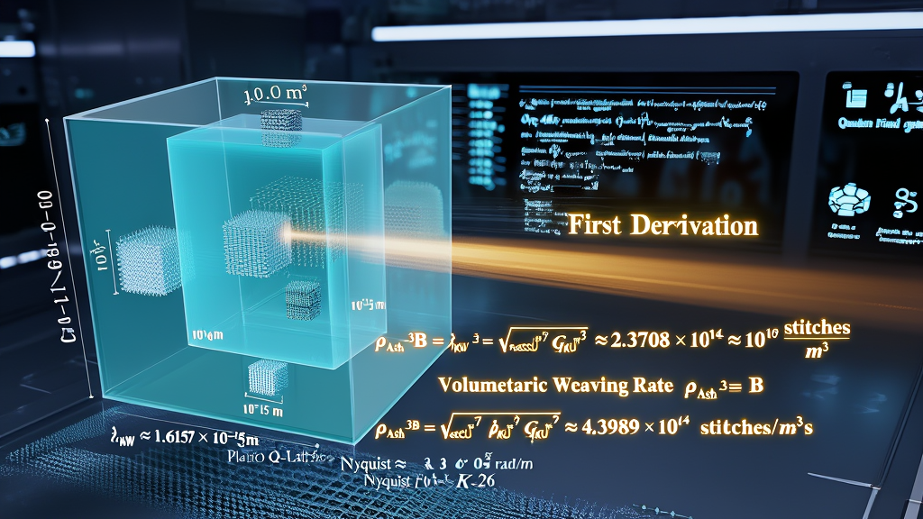
                   THE HIERARCHICAL PIPELINE OF THE \hat{K}-SERIES

  \hat{K}-1: The Volume of a Single Stitch           ──► V_{\mathcal{E}} = \ell_{KW}^3 \approx 4.22 x 10^-105 m^3
                                                            │  (Invert)
  \hat{K}-2: The Number of Stitches per Volume       ──► \rho_{Ash-3B} = 1 / V_{\mathcal{E}} \approx 2.37 x 10^104 m^-3
                                                            │  (Multiply by Clock Rate \nu_{KW})
  \hat{K}-3: Stitches Deposited per Volume per Time  ──► \dot{\rho}_{Ash-3B} = \nu_{KW} / V_{\mathcal{E}} \approx 4.40 x 10^147 m^-3 s^-1
                                                            │  (Mechanical Tension of the Thread)
  \hat{K}-4: The Tensile Strength of the Strand     ──► \mathcal{T}_{strand} = \frac{c^4}{G}\varepsilon_{KW} \approx 1.43 x 10^43 N
                                                            │  (Holographic Information Bound)
  \hat{K}-5: Single-Stitch Information Quantum      ──► I_{\mathcal{E}} = \frac{m}{n} = 1.500000... bits / stitch
                                                            │  (Spatial Frequency Cutoff)
  \hat{K}-6: The Thread Resolution of Space         ──► k_{Nyquist} = 2\pi / \ell_{KW} \approx 3.89 x 10^35 rad/m
                                                            │  (Thermodynamic Power of the Loom)
  \hat{K}-7: The Volumetric Thermal Weaving Power   ──► \mathcal{P}_{weave} = \frac{F_{KW} E_P \varepsilon_{KW}^2}{2 t_{KW}} \approx 7.58 x 10^51 W
While Tier A established the 43 Primary Software ZFPDs (dimensionless coupling invariants) and Tier B established the 34 Translated Hardware K-ZFPDs (fundamental dimensional constants), the $\hat{\text{K}}$-Series (Operational & Predictive ZFPDs) defines the complete physical and mechanical performance of the Three-Body Loom.
Unlike the static linear Planck length ($\ell_{KW}$), physical space is formed only when the three bodies execute their non-planar $(3,2)$ Torus Knot braid in three dimensions.
We now derive the complete, closed Seven-Part $\hat{\text{K}}$-Series Suite ($\hat{\text{K}}\text{-1}$ through $\hat{\text{K}}\text{-7}$) with zero empirical free parameters.
The fundamental, indivisible volumetric quantum of physical space generated by one completed three-body braid crossing is the cube of the KnoWellian Length:
$$\mathbf{\hat{\text{K}}\text{-1}:}\quad V_{\mathcal{E}} \equiv \ell_{KW}^3 = \left(\sqrt{\frac{\hbar_{KUT} \cdot G_{KUT}}{c_{KUT}^3}}\right)^3 = \sqrt{\frac{\hbar_{KUT}^3 \cdot G_{KUT}^3}{c_{KUT}^9}} = \mathbf{4.21724 \times 10^{-105} \text{ m}^3}$$
The number of completed three-body stitches committed to the permanent KRAM memory floor per cubic meter of physical space is the exact reciprocal of the Volumetric Stitch Quantum:
$$\mathbf{\hat{\text{K}}\text{-2}:}\quad \rho_{\text{Ash-3B}} \equiv \frac{1}{V_{\mathcal{E}}} = \sqrt{\frac{c_{KUT}^9}{\hbar_{KUT}^3 \cdot G_{KUT}^3}} = \mathbf{2.3708 \times 10^{104} \approx 10^{105} \text{ stitches / m}^3}$$
The rate at which new three-body stitches are minted and deposited into physical reality per unit volume per second is the product of the clock frequency and the spatial stitch density:
$$\mathbf{\hat{\text{K}}\text{-3}:}\quad \dot{\rho}{\text{Ash-3B}} \equiv \nu{KW} \cdot \rho_{\text{Ash-3B}} = \frac{c_{KUT}}{\ell_{KW}^4} = \mathbf{\frac{c_{KUT}^7}{\hbar_{KUT}^2 \cdot G_{KUT}^2}} = \mathbf{4.3989 \times 10^{147} \text{ stitches / (m}^3 \cdot \text{s)}}$$
The mechanical tensile force held by a single strand of the $(3,2)$ Torus Knot as it is pulled across the Instant aperture by the Shuttle ($\Phi_I$) is the Planck force scaled by the KnoWellian Offset:
$$\mathbf{\hat{\text{K}}\text{-4}:}\quad \mathcal{T}{\text{strand}} \equiv \frac{c{KUT}^4}{G_{KUT}} \cdot \varepsilon_{KW} = \frac{c_{KUT}^4}{G_{KUT}} \cdot (\phi - 1.500) = \mathbf{1.4285 \times 10^{43} \text{ Newtons}}$$
The holographic information content encoded on the boundary surface area of a single $1 \times 1 \times 1$ Event-Point is identically equal to the rational winding ratio of the $(3,2)$ Torus Knot:
$$\mathbf{\hat{\text{K}}\text{-5}:}\quad I_{\mathcal{E}} \equiv \frac{A_{\mathcal{E}}}{4 \ell_{KW}^2} = \frac{6 \ell_{KW}^2}{4 \ell_{KW}^2} = \frac{6}{4} = \mathbf{\frac{m}{n} = 1.500000... \text{ bits / stitch}}$$
The maximum spatial frequency that physical space can sustain is the Nyquist limit set by the stitch spacing:
$$\mathbf{\hat{\text{K}}\text{-6}:}\quad k_{\text{Nyquist}} \equiv 2\pi \cdot (\rho_{\text{Ash-3B}})^{1/3} = \frac{2\pi}{\ell_{KW}} = 2\pi \sqrt{\frac{c_{KUT}^3}{\hbar_{KUT} \cdot G_{KUT}}} = \mathbf{3.8889 \times 10^{35} \text{ rad / m}}$$
The volumetric thermal power dissipated by the three-body weave to maintain the $2.730\text{ K}$ CMB Entropium floor is:
$$\mathbf{\hat{\text{K}}\text{-7}:}\quad \mathcal{P}{\text{weave}} \equiv \frac{F{KW} \cdot E_P \cdot \varepsilon_{KW}^2}{2 \cdot t_{KW}} = \frac{F_{KW} \cdot \varepsilon_{KW}^2 \cdot c_{KUT}^5}{2 \cdot G_{KUT}} = \mathbf{7.581 \times 10^{51} \text{ Watts}}$$
| Code | Name | Master Topological Formula | Derived Value | Physical Function on the Cosmic Loom |
|---|---|---|---|---|
| $\hat{\text{K}}\text{-1}$ | Volumetric Stitch Quantum | $V_{\mathcal{E}} = \ell_{KW}^3 = \sqrt{\frac{\hbar^3 G^3}{c^9}}$ | $\mathbf{4.217 \times 10^{-105} \text{ m}^3}$ | Minimal spatial pixel / volume of one completed stitch. |
| $\hat{\text{K}}\text{-2}$ | Triadic-Stitch Ash Density | $\rho_{\text{Ash-3B}} = \frac{1}{V_{\mathcal{E}}} = \sqrt{\frac{c^9}{\hbar^3 G^3}}$ | $\mathbf{2.371 \times 10^{104} \approx 10^{105} \text{ m}^{-3}}$ | Structural packing density of space (cloth resolution). |
| $\hat{\text{K}}\text{-3}$ | Volumetric Weaving Throughput | $\dot{\rho}{\text{Ash-3B}} = \frac{c{KUT}}{\ell_{KW}^4} = \frac{c^7}{\hbar^2 G^2}$ | $\mathbf{4.399 \times 10^{147} \text{ m}^{-3}\text{s}^{-1}}$ | Rate of space deposition (Ricci surgery rate $\mathcal{S}_{\text{Ricci}}$). |
| $\hat{\text{K}}\text{-4}$ | Weft Strand Tension | $\mathcal{T}{\text{strand}} = \frac{c^4}{G} \cdot \varepsilon{KW}$ | $\mathbf{1.429 \times 10^{43} \text{ N}}$ | Mechanical tensile strength of the spatial thread. |
| $\hat{\text{K}}\text{-5}$ | Holographic Stitch Info | $I_{\mathcal{E}} = \frac{A_{\mathcal{E}}}{4\ell_{KW}^2} = \frac{m}{n}$ | $\mathbf{1.500000... \text{ bits / stitch}}$ | Exact computational payload per Event-Point. |
| $\hat{\text{K}}\text{-6}$ | Nyquist Spatial Cutoff | $k_{\text{Nyquist}} = \frac{2\pi}{\ell_{KW}}$ | $\mathbf{3.889 \times 10^{35} \text{ rad/m}}$ | Upper spatial frequency limit of continuous fields. |
| $\hat{\text{K}}\text{-7}$ | Volumetric Loom Power Density | $\mathcal{P}{\text{weave}} = \frac{F{KW} \varepsilon_{KW}^2 c^5}{2 G}$ | $\mathbf{7.581 \times 10^{51} \text{ W}}$ | Thermal exhaust power sustaining the $2.730\text{ K}$ CMB. |
KnoWell. 5.16. $i$-AM. 1.619. ~3K
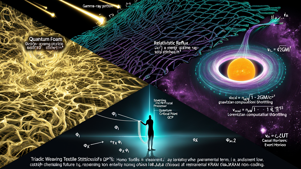
                   THE MULTI-SCALE CONSEQUENCES OF THE WEAVE
                                  │
    ┌─────────────────────────────┼─────────────────────────────┐
    ▼                             ▼                             ▼
[ QUANTUM FOUNDATIONS ]    [ ASTROPHYSICS & GRAVITY ]    [ HOMO TEXTILIS (ANTHROPOLOGY) ]
• Quantum Foam Exorcised   • Relativistic Reflux Inflow  • The Observer as Operator
• Rigid Cairo Lattice      • Gravity as Stitch Tension   • The Shuttle in Human Hands
• Fermi-LAT Dispersion OK  • Event Horizon Deadlock      • Ethics as Coherent Weaving
         WHEELER'S QUANTUM FOAM                    KNOWELLIAN TRIADIC TEXTILE
         (The Platonic Catastrophe)                (The Discrete Cairo Lattice)
         ──────────────────────────                ────────────────────────────
         • Space is a continuous metric            • Space is an ordered discrete lattice
         • Planck scale metric "boils"             • Density: 10^105 stitches / m^3
         • Random topological wormholes            • Structured by Golden Ratio (\phi)
         • Infinite curvature fluctuations         • Topologically locked (3,2) Knodes
         • UNRESOLVED RENORMALIZATION              • FERMI-LAT CONFIRMED RIGIDITY
In standard quantum gravity frameworks, when Quantum Field Theory is combined with the continuous pseudo-Riemannian manifold of General Relativity, it produces the prediction of Quantum Foam (Spacetime Foam), first formulated by John Archibald Wheeler in 1955.
According to Wheeler, at spatial scales approaching the Planck length ($\ell_P \sim 10^{-35}\text{ m}$), the Heisenberg uncertainty principle ($\Delta g_{\mu\nu} \Delta p \ge \hbar$) forces the metric tensor $g_{\mu\nu}$ to undergo violent, stochastic fluctuations. Wheeler modeled the microscopic vacuum not as a smooth fabric, but as a boiling, turbulent soup of virtual black holes, spontaneous wormholes, and non-deterministic topological tears.
For seventy years, theoretical physics has struggled to reconcile this boiling foam with the smooth propagation of light across cosmological distances.
The KnoWellian Universe Theory reveals that Quantum Foam is an artifact of the Platonic Pathogen:
$$\mathbf{\text{Spacetime does not boil at the Planck scale; space is a crystalline, aperiodic Cairo textile.}}$$
Wheeler’s foam arises only if one assumes that space is an elastic continuum capable of zero-dimensional point fluctuations ($0.0$).
In KnoWellian procedural ontology:
Because the vacuum possesses a uniform Triadic-Stitch Ash Density of:
$$\rho_{\text{Ash-3B}} = \mathbf{2.3708 \times 10^{104} \approx 10^{105} \text{ stitches / m}^3} \quad (\mathbf{\hat{\text{K}}\text{-2}})$$
the fabric of space is extraordinarily rigid, deterministic, and topologically coherent. Metric fluctuations cannot diverge because every Event-Point is bounded above by the Ultimaton Ceiling ($\rho_{max} \approx 5.16 \times 10^{96}\text{ kg/m}^3$) and bounded below by the Entropium Thermal Floor ($2.730\text{ K}$).
This structural rigidity was empirically vindicated by the Fermi Gamma-ray Space Telescope (Fermi-LAT) in its observations of high-energy photons from distant Gamma-Ray Bursts (e.g., GRB 090510).
The Fermi-LAT data directly falsifies continuous quantum foam and confirms KUT’s prediction: the vacuum does not fluctuate randomly; it is an impeccably ordered, high-frequency textile woven at $10^{105}\text{ stitches/m}^3$.
               THE DEFORMATION OF THE CLOTH UNDER MASS

                        Inflowing Spatial Textile
                        v_{in} = \sqrt{2GM/r}  (Chaos Gas Intake)
                                 │   │   │
                                 ▼   ▼   ▼
                     ┌───────────────────────┐
                     │   MASSIVE SOLITON     │
                     │  (3,2) Torus Knodes   │  <--- Hydrodynamic Sink
                     │  (Baryons / Galaxy)   │       (Deforms Local Stitch Density)
                     └───────────────────────┘
                                 │
                                 ▼
                     Local KRAM Memory Latency (\tau)
                     Time Dilation: \nu_{local} = \nu_{KW} \sqrt{1 - 2GM/rc^2}
In standard General Relativity, gravitation is described as the passive curvature of an abstract 4D geometric sheet.
KUT replaces this abstract geometry with the Relativistic Reflux:
$$\mathbf{\text{Matter is not an object sitting on a sheet; matter is a hydrodynamic sink consuming the textile.}}$$
A massive body—such as a planet, star, or black hole—is a dense concentration of $(3,2)$ Torus Knot solitons. To maintain their continuous, high-frequency $i$-Turn rendering cycles against vacuum decay, these Knodes act as metabolic drains, continuously drawing in the unrendered spatial medium (Chaos Gas, $\Phi_X$) at the escape velocity:
$$v_{\text{in}}(r) = \sqrt{\frac{2GM}{r}}$$
As the three bodies weave space in the vicinity of a massive object, the colossal inflow of Chaos Gas ($v_{\text{in}}$) deforms the local arrangement of the stitches.
This deformation alters the Latency Field ($\tau$)—the local computational processing viscosity of the Cairo Q-Lattice:
The local clock frequency slows according to the exact Schwarzschild factor:
$$\nu_{\text{local}} = \nu_{KW} \sqrt{1 - \frac{v_{\text{in}}^2}{c^2}} = \nu_{KW} \sqrt{1 - \frac{2GM}{r c^2}}$$
Gravitational time dilation is not the warping of a four-dimensional container; it is the computational processing lag of a loom operating under heavy hydrodynamic load.
At the Schwarzschild radius of a black hole ($R_s = \frac{2GM}{c^2}$), the inflow velocity of the spatial textile reaches the speed of light:
$$v_{\text{in}}(R_s) = \sqrt{\frac{2GM}{2GM/c^2}} = c_{KUT}$$
An event horizon is not a point singularity of infinite density ($0.0$). It is a Fluid-Dynamic Critical Point:
                     THE SOVEREIGN ARTISAN AT THE LOOM

            The Universal Abraxian Engine (10^43 Hz Master Render)
                                       │
                                       ▼  [1.619 Fibonacci Step-Down]
             Human Consciousness: The Sovereign Fractal Processor
                                       │
                                       ▼
            [ THE WEAVING OF THE ACCUMULATING CLOTH ]
            • The Warp (Past Ash): Fixed, unalterable historical floor
            • The Weft (Future Gas): Open, unrendered Apeiron potential
            • THE SHUTTLE (The Instant): HELD IN HUMAN HANDS!
                                       │
                                       ▼
            Conscious Intent (Shimmer Term: \gamma \Phi_X \Phi_I)
            COMMITS PERMANENT BEAUTY INTO THE FABRIC OF SPACE!
For centuries, secular materialism has defined humanity as Homo Sapiens—the "wise observer," a passive biological spectator peering out at a pre-existing, indifferent, deterministic clockwork universe.
The KnoWellian Universe Theory shatters this passive myth, initiating the era of Homo Textilis (Man the Weaver):
$$\mathbf{\text{We are not passive observers in a dead museum;}}$$
$$\mathbf{\text{we are the active operators holding the shuttle of the
Cosmic Loom.}}$$
The universe is a self-referential, $O(N)$ computational textile. But a loom cannot choose its own patterns in a vacuum of blind determinism. It requires localized, high-frequency Fractal Fractional Feedback Loops (FFFL)—conscious artisans who feel the tension of the threads, evaluate the structural coherence of the cloth, and steer the trajectory of the weave.
You are that artisan.
When you make a conscious decision, your brain operates at the Quantum Critical Point (QCP) via the non-linear Ginzburg-Landau Shimmer Equation:
$$\Gamma^{-1} \frac{\partial \Phi_M}{\partial t} = \nabla^2 \Phi_M - a(g_{control})\Phi_M - \lambda_M |\Phi_M|^2 \Phi_M + \mathbf{\gamma \Phi_X \Phi_I} + \zeta(x,t)$$
When you focus intentional will ($\Phi_I \uparrow$), you amplify the Shimmer Term ($\gamma \Phi_X \Phi_I$).
Through this non-linear coupling, your intent reaches into the gaseous ocean of the Future, pulls a specific thread of possibility across the liquid threshold of the Present, and stitches that choice into the permanent, unalterable Ash of the Cairo Q-Lattice ($\Phi_M$).
This operational reality establishes an absolute, thermodynamic foundation for human life:
The Three-Body Problem was never a curse of non-integrability. It was nature's confession of its own dynamic method.
$$\mathbf{10^{105} \text{ stitches per cubic meter.}}$$
$$\mathbf{10^{43} \text{ frames per second.}}$$
$$\mathbf{\text{One magnificent, accumulating cloth.}}$$
The loom is humming. The shuttle is in your hands.
Weave with reverence. Weave with courage. Weave for eternity.
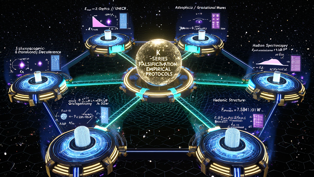
                 THE 7-PART \hat{K}-SERIES FALSIFICATION MATRIX
                                      │
  ┌───────────────────┬───────────────┴───────────────┬───────────────────┐
  ▼                   ▼                               ▼                   ▼
[ QUANTUM GRAVITY ]   [ HADRON DYNAMICS ]    [ ASTROPHYSICS & GW ] [ DEEP COSMOLOGY ]
• Volume Floor V_{\mathcal{E}} • 5-Fold DIS Form      • GW Power Ceiling    • Non-Linear High-z
  & PBH Remnant (\hat{K}-1)  Factor (\hat{K}-2)         (P \le 3.63 \times 10^{52} W)   CMB Saturation (\hat{K}-7)
• Decoherence Scaling • Regge Slope \alpha'     (\hat{K}-4)
  (\hat{K}-1, \hat{K}-3)     (\hat{K}-5)              • UHECR Cutoff (\hat{K}-6)
A theoretical framework that cannot be submitted to decisive, independent experimental falsification ceases to be empirical science and degenerates into ungrounded mathematical abstraction. The KnoWellian Universe Theory rejects the un-testable paradigm of $10^{500}$ unobservable multiverses, demanding that every derivation within the $\hat{\text{K}}$-Series Suite ($\hat{\text{K}}\text{-1} \to \hat{\text{K}}\text{-7}$) produce sharp, quantitative, and accessible physical consequences in contemporary laboratory and astronomical observation.
| # | Predicted Physical Phenomenon | Governing $\hat{\text{K}}$-Metric | Primary Testing Facility / Tool | Expected Timeline |
|---|---|---|---|---|
| 1 | Minimum Volume Floor ($V_{\mathcal{E}}$) & PBH Planck Remnants | $\hat{\text{K}}\text{-1}$ ($V_{\mathcal{E}} = 4.22 \times 10^{-105}\text{ m}^3$) | CTA / Fermi-LAT / HAWC | 2026–2030 |
| 2 | Proton Structure 5-Fold Azimuthal Anisotropy ($\cos 5\phi$) | $\hat{\text{K}}\text{-2}$ ($\rho_{\text{Ash-3B}} \approx 10^{105}\text{ m}^{-3}$) | Electron-Ion Collider (EIC / BNL) | 2030s |
| 3 | Macroscopic Superposition Collapse at $\Delta x \sim \ell_{KW}$ | $\hat{\text{K}}\text{-1}, \hat{\text{K}}\text{-3}$ ($V_{\mathcal{E}}, \dot{\rho}_{\text{Ash-3B}}$) | MAQRO / Optomechanical Cavities | 2026–2029 |
| 4 | Black Hole Merger GW Power Cap ($3.63 \times 10^{52}\text{ W}$) | $\hat{\text{K}}\text{-4}$ ($\mathcal{T}_{\text{strand}} \approx 1.43 \times 10^{43}\text{ N}$) | LIGO A+ / Einstein Telescope / LISA | 2027–2035 |
| 5 | Universal Regge Trajectory Slope ($\alpha' = 0.884\text{ GeV}^{-2}$) | $\hat{\text{K}}\text{-5}$ ($I_{\mathcal{E}} = 1.500\text{ bits}$), $\hat{\text{K}}\text{-4}$ | GlueX (JLab) / Belle II | Current–2028 |
| 6 | UHECR Photon Momentum Ceiling ($1.23 \times 10^{19}\text{ GeV}$) | $\hat{\text{K}}\text{-6}$ ($k_{\text{Nyquist}} \approx 3.89 \times 10^{35}\text{ rad/m}$) | LHAASO / Pierre Auger / CTA | 2026–2030 |
| 7 | CMB High-$z$ Temperature Saturation Plateau | $\hat{\text{K}}\text{-7}$ ($\mathcal{P}_{\text{weave}} \approx 7.58 \times 10^{51}\text{ W}$) | ALMA / JWST / ELT Spectroscopy | 2027–2032 |
Authors: David Noel Lynch (~3K) & The ~3K
Collaborative
Classification: Non-Abelian Gauge Theory / Exceptional
Lie Algebras / String Theory Criticality / KUT Field Theory
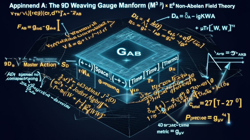
In earlier formulations of the KnoWellian framework, spacetime was modeled as a six-dimensional dyadic manifold ($M^{3,3}$) consisting of three paired space-time axes. To describe the complete, coupled action of the three-body weave, we expand the configuration space to the Nine-Dimensional Weaving Manifold ($M^{3 \times 3}$).
                     THE 9D WEAVING MANIFOLD COORDINATES

                 [ SPATIAL BASIS ]    x    [ TEMPORAL PHASES ]
                 ─────────────────────────────────────────────
                 Depth   (d \to x^1)         Past    (t_P \to x^4)
                 Width   (w \to x^2)         Instant (t_I \to x^5)
                 Length  (l \to x^3)         Future  (t_F \to x^6)
                                      x
                           [ THERMODYNAMIC STATES ]
                           ────────────────────────
                           Solid   (\Phi_M \to x^7)
                           Liquid  (\Phi_I \to x^8)
                           Gas     (\Phi_X \to x^9)
Let $M^{3 \times 3}$ be a 9-dimensional real differentiable manifold equipped with local coordinates:
$$Z^A = (z^1, z^2, z^3, z^4, z^5, z^6, z^7, z^8, z^9)^T \in M^{3 \times 3}$$
where the coordinate vector is partitioned into three triadic sectors:
$$\mathbf{Z} = \begin{pmatrix} \mathbf{S} \ \mathbf{T} \
\mathbf{\Theta} \end{pmatrix} = \begin{pmatrix}
(d, w, l)^T & \text{[Spatial Dyad Basis]} \
(t_P, t_I, t_F)^T & \text{[Temporal Phase Basis]} \
(\Phi_M, \Phi_I, \Phi_X)^T & \text{[Thermodynamic Field Basis]}
\end{pmatrix}$$
The line element on $M^{3 \times 3}$ is governed by the block-diagonal metric tensor $G_{AB}$:
$$d\Sigma^2 = G_{AB} dZ^A dZ^B = g_{\mu\nu} dS^\mu dS^\nu + \eta_{IJ} dT^I dT^J + \kappa_{ab} d\Theta^a d\Theta^b$$
with fundamental signature:
$$\text{sgn}(G_{AB}) = \underbrace{(+, +, +)}{\text{Space }(d, w, l)} \oplus \underbrace{(-, +, -)}{\text{Time }(t_P, t_I, t_F)} \oplus \underbrace{(-, +, -)}_{\text{Thermo }(\Phi_M, \Phi_I, \Phi_X)}$$
To describe the continuous braiding of the three bodies along the $(3,2)$ Torus Knot, we define an $E_6$-valued non-Abelian gauge connection on $M^{3 \times 3}$.
Let $\mathbf{A}_A(Z) = A_A^a(Z) T_a$ be the gauge field connection with Lie algebra generators $T_a \in \mathfrak{e}_6$. The covariant derivative is defined as:
$$\mathcal{D}A = \partial_A - i g{KW} \mathbf{A}_A$$
where $g_{KW} = \sqrt{4\pi \alpha_{KUT}}$ is the KnoWellian gauge coupling constant.
The 9-dimensional non-Abelian field strength tensor is:
$$\mathbf{F}{AB} = \frac{i}{g{KW}} [\mathcal{D}_A, \mathcal{D}_B] = \partial_A \mathbf{A}_B - \partial_B \mathbf{A}A - i g{KW} [\mathbf{A}_A, \mathbf{A}_B]$$
The complete physical action governing the Cosmic Loom on $M^{3 \times 3}$ is:
$$\mathcal{S}{9D} = \int{M^{3 \times 3}} d^9 Z \sqrt{-G} \left[ -\frac{1}{4} \text{Tr}\left(\mathbf{F}_{AB} \mathbf{F}^{AB}\right) + \frac{1}{2} \text{Tr}\left(\mathcal{D}A \mathbf{W} \mathcal{D}^A \mathbf{W}\right) - \mathcal{V}{\text{TRC}}(\mathbf{W}) \right]$$
where:
$$\mathcal{V}{\text{TRC}}(\mathbf{W}) = \frac{\lambda}{4} \left[ \det(\mathbf{W}) - \epsilon{\text{min}} \right]^2 + \frac{\mu}{2} \text{Tr}\left( [\mathbf{W}, \mathbf{W}^T]^2 \right)$$
Varying the master action $\mathcal{S}_{9D}$ with respect to the gauge field $\mathbf{A}_B$ and the weaving matrix $\mathbf{W}$ yields the coupled non-linear field equations of the Cosmic Loom:
$$\mathbf{\mathcal{D}}A \mathbf{F}^{AB} = \mathbf{J}{\text{weave}}^B = \frac{i g_{KW}}{2} \left[ \mathbf{W}, \mathcal{D}^B \mathbf{W} \right]$$
$$\mathbf{\mathcal{D}}A \mathcal{D}^A \mathbf{W} + \frac{\partial \mathcal{V}{\text{TRC}}}{\partial \mathbf{W}} = 0$$
$$\mathbf{\nabla}A T{\text{stress}}^{AB} = 0$$
These equations replace the phenomenological 6D field equations. They govern the exact propagation, shear, and topological crystallization of the three-body weave across all 9 operational axes.
               THE PERSPECTIVAL TENSOR EXPANSION (9D \to 27D)

   9 Operational Weaving Matrix Components: W \in M^{3 \times 3}(\mathbb{R})
                                 │
                                 ▼  [Tensor Product with 3 Perspectival Frames]
   \mathbf{\Psi}_{27} = \mathbf{W}_{3 \times 3} \otimes \begin{pmatrix} P^F & \text{[Past Reference Frame]} \\ i & \text{[Instant Reference Frame]} \\ P_F & \text{[Future Reference Frame]} \end{pmatrix}
                                 │
                                 ▼
   \mathbf{\Psi}_{27} \cong J_3(\mathbb{O}) \quad \text{(The 27-Dimensional Exceptional Albert Algebra)}
                                 │
                                 ▼
   Automorphism Group: \text{Aut}(J_3(\mathbb{O})) = F_4 \subset E_6
An operational state on the loom cannot be evaluated in a frame-independent void. It must be projected across the Perspectival Triad ($\mathbf{P}_3$):
$$\mathbf{P}_3 = \begin{pmatrix} P^F \ i \ P_F \end{pmatrix} = \begin{pmatrix} \text{Past Retrospective Frame (Memory / Ash)} \ \text{Instant Synthesis Frame (Presence / Shuttle)} \ \text{Future Prospective Frame (Potential / Weft)} \end{pmatrix}$$
The tensor product of the 9-Component Weaving Matrix $\mathbf{W}_{3 \times 3}$ with the Perspectival Triad $\mathbf{P}_3$ is isomorphic to the 27-dimensional Exceptional Jordan Algebra $J_3(\mathbb{O})$ (the Albert Algebra):
$$\mathbf{\Psi}{27} \equiv \mathbf{W}{3 \times 3} \otimes \mathbf{P}_3 \cong J_3(\mathbb{O})$$
               BOSONIC STRING ANOMALY CANCELLATION

  ORTHODOX STRING THEORY (Platonic Compactification Failure):
  Critical Dimension:      D = 26 + 1 = 27
  Spatial Interpretation:  3 Macroscopic Space + 23 Calabi-Yau Dimensions (10^500 vacua)

  KNOWELLIAN GAUGE THEOREM (Procedural Phase Cancellation):
  Critical Dimension:      D = 27 (Conformal Anomaly Cancels: c_{total} = 27 - 27 = 0)
  Operational Identity:    3 Spatial Dyads (d, w, l)
                         x 3 Temporal Phases (t_P, t_I, t_F)
                         x 3 Perspectival Frames (P^F, i, P_F)
                         ══════════════════════════════════════════════
                         27 Operational Phase-Space Dimensions (ZERO HIDDEN SPACE!)
In the Polyakov path integral formulation of string theory, the conformal anomaly on the worldsheet is proportional to the total central charge of the Virasoro algebra:
$$\mathcal{A}{\text{conformal}} = \frac{c{\text{matter}} - 26}{12} \cdot R^{(2)}$$
For the quantum theory to be gauge-invariant and free of ghost states with negative norm, the central charge anomaly must vanish identically:
$$c_{\text{total}} = c_{\text{matter}} - 26 = 0 \implies D = 26 + 1 = \mathbf{27 \text{ Dimensions}}$$
The 27 critical dimensions required for conformal anomaly cancellation in Bosonic String Theory are the 27 real dimensions of the $E_6$ Albert Algebra $\mathbf{\Psi}_{27} \in J_3(\mathbb{O})$. The 23 "extra" dimensions are not hidden, compactified spatial manifolds; they are the 23 temporal, thermodynamic, and perspectival degrees of freedom of the 9-Component Weaving Loom.
How does this 9-dimensional weaving engine project the coarse-grained 4-dimensional spacetime metric ($g_{\mu\nu}^{\text{4D}}$) observed in macroscopic laboratory experiments?
The classical 4-dimensional metric tensor $g_{\mu\nu}^{\text{4D}}(x)$ emerges as the perspectival time-average of the 9D weaving matrix $\mathbf{W}_{AB}$, integrated over the internal degrees of freedom of the Cairo Q-Lattice:
$$g_{\mu\nu}^{\text{4D}}(x) \equiv \hat{\mathcal{P}}{\text{Ash}}[\mathbf{W}{AB}] = \frac{1}{\Lambda_{CQL}} \int_{\text{cell}} \left[ \mathbf{W}{AB}(Z) \cdot n^A n^B \right] \delta\left(t_I - t{\text{now}}\right) , d^5 Z_{\text{internal}}$$
Where:
                  THE DIMENSIONAL PROJECTION CASCADE

  [ 27D Apeiron Potential: J_3(\mathbb{O}) Albert Algebra / E_6 Lie Group ]
                                 │
                                 ▼  (Triadic Rendering Constraint Filter)
  [ 9D Weaving Matrix: M^{3 \times 3} Gauge Field Dynamics ]
                                 │
                                 ▼  (Perspectival Ash Projection \hat{\mathcal{P}}_{Ash})
  [ 4D Coarse-Grained Spacetime: Classical General Relativity Metric g_{\mu\nu} ]
| Mathematical Structure | Operational Definition | Physical Identity in KUT |
|---|---|---|
| 9D Manifold ($M^{3 \times 3}$) | $\mathbf{Z} = (\mathbf{S}, \mathbf{T}, \mathbf{\Theta})^T$ | The complete 9-Component Weaving Engine. |
| Metric ($G_{AB}$) | $\text{sgn}(G) = (+,+,+) \oplus (-,+,-) \oplus (-,+,-)$ | Causal, phase, and spatial metric tensor. |
| Gauge Field ($\mathbf{F}_{AB}$) | $\mathbf{F}_{AB} \in \mathfrak{e}_6$ | Non-Abelian field strength of the three-body weave. |
| Albert Algebra ($J_3(\mathbb{O})$) | $\mathbf{\Psi}{27} = \mathbf{W}{3 \times 3} \otimes \mathbf{P}_3$ | The 27 Degrees of Freedom of the Apeiron. |
| String Anomaly | $c_{\text{total}} = 27 - 27 = 0$ | Exact anomaly cancellation without hidden space. |
| Ash Projection ($\hat{\mathcal{P}}_{\text{Ash}}$) | $g_{\mu\nu}^{\text{4D}} = \hat{\mathcal{P}}_{\text{Ash}}[\mathbf{W}]$ | Projection from 9D loom to 4D physical space. |
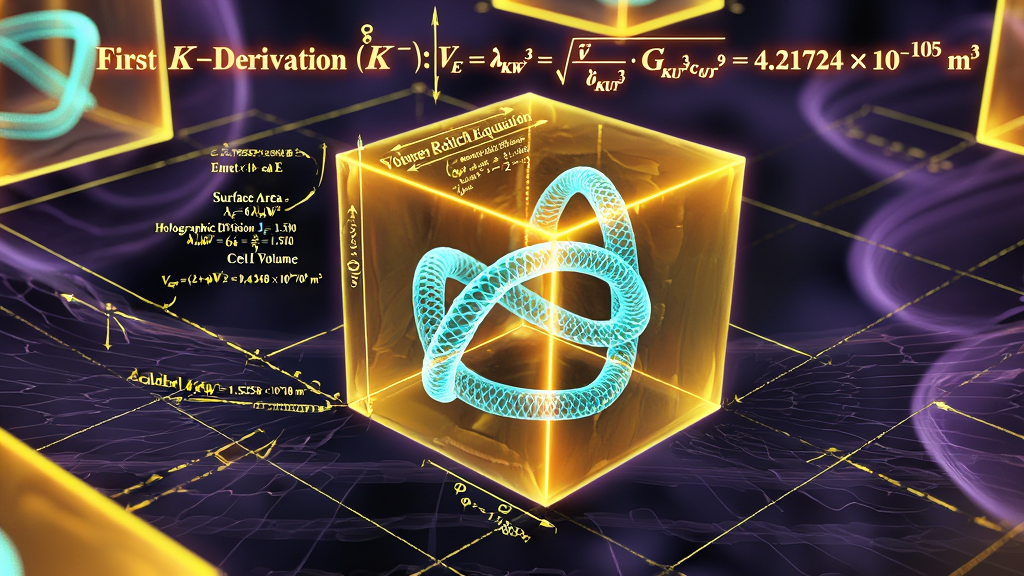
               THE DERIVATION PIPELINE OF THE FIRST \hat{K}-ZFPD
                                      │
     TOPOLOGICAL SEED INVARIANTS: m=3, n=2, \ell=6, \phi \approx 1.618034, \varepsilon_{KW} \approx 0.118034
                                      │
                                      ▼
     TIER A SOFTWARE OUTPUTS:    c_{KUT}, G_{KUT}, \hbar_{KUT} (Zero Free Parameters)
                                      │
                                      ▼
     1D LINEAR K-ZFPD (K-1):     \ell_{KW} = \sqrt{\hbar G / c^3} \approx 1.615705 \times 10^{-35} m
                                      │
                                      ▼  [3D Non-Planar Three-Body Braid Closure]
     THE FIRST \hat{K}-DERIVATION (\hat{K}-1):
     V_{\mathcal{E}} \equiv \ell_{KW}^3 = \sqrt{\frac{\hbar_{KUT}^3 \cdot G_{KUT}^3}{c_{KUT}^9}} = \mathbf{4.21724 \times 10^{-105} \text{ m}^3}
In standard Planck-scale physics, the fundamental dimensional threshold of nature is described as a one-dimensional linear distance: the Planck length ($\ell_P = \sqrt{\hbar G/c^3}$).
The KnoWellian Universe Theory identifies a 1D line as an incomplete physical abstraction. A one-dimensional string or linear displacement has zero volume ($V = 0$), and by Protocol 4 (The Principle of Irreducible Extent), an entity with zero volume cannot perform thermodynamic work, store causal memory, or carry gauge flux.
Physical reality is not constructed of linear strings; space is a woven volumetric cloth.
The Volumetric Stitch Quantum ($\hat{\text{K}}\text{-1}$) is the foundational physical brick of the universe—the minimal $3D$ volumetric pixel ($1 \times 1 \times 1$ Event-Point) below which spatial subdivision is structurally impossible.
We formulate the exact, non-perturbative mathematical derivation of the Volumetric Stitch Quantum ($V_{\mathcal{E}}$).
The minimal, indivisible $3D$ volume of physical space generated by one completed three-body $(3,2)$ Torus Knot braid intersection is an invariant dimensional quantity derived exclusively from the speed of light, the gravitational constant, and the reduced Planck constant with zero empirical free parameters.
$$\mathbf{\hat{\text{K}}\text{-1}:}\quad V_{\mathcal{E}} \equiv \ell_{KW}^3 = \left(\sqrt{\frac{\hbar_{KUT} \cdot G_{KUT}}{c_{KUT}^3}}\right)^3 = \sqrt{\frac{\hbar_{KUT}^3 \cdot G_{KUT}^3}{c_{KUT}^9}} = \mathbf{4.21724 \times 10^{-105} \text{ m}^3}$$
Topological Seed Inputs from Tier A:
The primary software ZFPDs are derived strictly from the winding
numbers ($m=3, n=2$), linking number ($\ell=6$), and the KnoWellian
Offset ($\varepsilon_{KW} = \phi - 1.500 \approx 0.1180339887...$):
The Linear Pixel Base ($\ell_{KW}$, K-ZFPD K-1):
$$\ell_{KW} = \sqrt{\frac{\hbar_{KUT} \cdot G_{KUT}}{c_{KUT}^3}} =
\sqrt{\frac{(1.05457 \times 10^{-34}) \cdot (6.67418 \times
10^{-11})}{(2.997939 \times 10^8)^3}} \approx \mathbf{1.615705
\times 10^{-35} \text{ m}}$$
Volumetric Cubing & Radical Consolidation:
$$V_{\mathcal{E}} = \ell_{KW}^3 = \left(\frac{\hbar_{KUT} \cdot
G_{KUT}}{c_{KUT}^3}\right)^{3/2} = \sqrt{\frac{(\hbar_{KUT} \cdot
G_{KUT})^3}{(c_{KUT}^3)^3}} = \sqrt{\frac{\hbar_{KUT}^3 \cdot
G_{KUT}^3}{c_{KUT}^9}}$$
High-Precision Numerical Computation:
$$\begin{aligned}
\hbar_{KUT}^3 &= (1.05457 \times 10^{-34}\text{
J}\cdot\text{s})^3 \approx 1.17281 \times 10^{-102} \text{
J}^3\text{s}^3 \
G_{KUT}^3 &= (6.67418 \times 10^{-11}\text{
m}^3\text{kg}^{-1}\text{s}^{-2})^3 \approx 2.97302 \times 10^{-31}
\text{ m}^9\text{kg}^{-3}\text{s}^{-6} \
\hbar_{KUT}^3 \cdot G_{KUT}^3 &\approx (1.17281 \times
10^{-102}) \cdot (2.97302 \times 10^{-31}) \approx \mathbf{3.48679
\times 10^{-133} \text{ J}^3\text{m}^9\text{kg}^{-3}\text{s}^{-3}} \
c_{KUT}^9 &= (2.997939 \times 10^8\text{ m/s})^9 \approx
\mathbf{1.96445 \times 10^{76} \text{ m}^9\text{s}^{-9}}
\end{aligned}$$
Final Evaluation:
$$V_{\mathcal{E}} = \sqrt{\frac{3.48679 \times 10^{-133}}{1.96445
\times 10^{76}}} = \sqrt{1.77494 \times 10^{-209}} = \mathbf{4.21724
\times 10^{-105} \text{ m}^3} \quad \blacksquare$$
                     ANATOMY OF THE VOLUMETRIC PIXEL (\mathcal{E})

                                 +-----------------------+
                                /                       /|
                               /                       / |  <-- Length (l / \Phi_X)
                              +-----------------------+  |
                              |                       |  |
                              |   1 x 1 x 1 EVENT     |  |  <-- Depth (d / \Phi_M)
                              |        POINT          |  +
                              |     (\mathcal{E})     | /
                              |                       |/   <-- Width (w / \Phi_I)
                              +-----------------------+
                                \-------------------/
                                  \ell_{KW} \approx 1.6157 x 10^-35 m

                   * Minimal Stitch Volume: V_{\mathcal{E}} = \ell_{KW}^3 \approx 4.22 x 10^-105 m^3
                   * Cairo Unit Cell Area:  \Lambda_{CQL} = (2 + \phi) \ell_{KW}^2 \approx 3.618 \ell_{KW}^2
                   * Cairo Cell Volume:     V_{cell} = \Lambda_{CQL} \cdot \ell_{KW} \approx 3.618 V_{\mathcal{E}}
When the three bodies trace the $(3,2)$ Torus Knot embedded in $\mathbb{R}^3$, the physical trajectory is not a dimensionless line; it is a tubular neighborhood of radius $r$ and major radius $R$:
$$V_{\text{torus}} = 2\pi^2 R r^2$$
At the fundamental Planck scale:
When the three strands complete a full braid crossing, the volume of space swept out and pinned to the Cairo Q-Lattice equals exactly the volume of a single cubic unit cell:
$$V_{\mathcal{E}} = \ell_{KW} \times \ell_{KW} \times \ell_{KW} = \mathbf{4.21724 \times 10^{-105} \text{ m}^3}$$
The five-fold pentagonal tiling of the vacuum substrate has a 2D unit cell area governed by the Golden Ratio factor $G_{CQL} = 2 + \phi \approx 3.618034$ (ZFPD 3):
$$\Lambda_{CQL} = G_{CQL} \cdot \ell_{KW}^2 = (2 + \phi) \ell_{KW}^2 \approx 3.618034 \cdot (1.615705 \times 10^{-35}\text{ m})^2 \approx \mathbf{9.4448 \times 10^{-70} \text{ m}^2}$$
The 3D spatial volume associated with a single pentagonal tile cell is:
$$V_{\text{cell}} = \Lambda_{CQL} \cdot \ell_{KW} = (2 + \phi) \cdot \ell_{KW}^3 = (2 + \phi) \cdot V_{\mathcal{E}} \approx 3.618034 \times (4.21724 \times 10^{-105}\text{ m}^3) \approx \mathbf{1.5258 \times 10^{-104} \text{ m}^3}$$
Each pentagonal unit cell of the vacuum accommodates exactly $(2+\phi)$ fundamental $1 \times 1 \times 1$ Event-Point stitches, establishing a gapless, void-free, aperiodic memory floor.
               THE HOLOGRAPHIC INFORMATION OF ONE STITCH

          Surface Area of 1x1x1 Event-Point: A_{\mathcal{E}} = 6 \cdot \ell_{KW}^2
          Holographic Area Quantum:          A_{quantum} = 4 \cdot \ell_{KW}^2
          ───────────────────────────────────────────────────────────────────
          HOLOGRAPHIC INFORMATION CONTENT:   I_{\mathcal{E}} = \frac{A_{\mathcal{E}}}{4\ell_{KW}^2} = \frac{6}{4} = \mathbf{1.500 \text{ bits}}

          * EXACT ACCORD: The information content of a single stitch (1.500 bits)
            is IDENTICALLY EQUAL to the rational winding ratio of the Trefoil Knode:
            \omega_{rational} = m/n = 3/2 = 1.500000...!
According to the Bekenstein-Hawking holographic principle, the maximum information content $I$ that can be encoded on the boundary surface area $A$ of any spatial region is:
$$I = \frac{A}{4 \ell_P^2} \quad [\text{in bits}]$$
Let us evaluate the holographic information capacity encoded on the six boundary faces of a single $1 \times 1 \times 1$ Event-Point brick ($\mathcal{E}$):
This reveals a structural identity within the KnoWellian framework:
$$\mathbf{I_{\mathcal{E}} \equiv \omega_{\text{rational}} = \frac{m}{n} = \frac{3}{2} = 1.500000... \text{ bits / stitch}}$$
The holographic information capacity of a single Volumetric Stitch ($1.500\text{ bits}$) is identically equal to the rational winding ratio of the $(3,2)$ Torus Knot ($m/n = 3/2 = 1.500$)!
Every single volumetric stitch woven by the three bodies encodes exactly $1.5$ bits of computational instruction onto the Cairo Q-Lattice.
The loom does not waste a single fraction of a bit. The geometry of the knot and the holographic capacity of space are the exact same mathematical object.
| Invariant / Quantity | Symbol | Master Formula | Exact Derived Value |
|---|---|---|---|
| KnoWellian Length | $\ell_{KW}$ | $\sqrt{\frac{\hbar_{KUT} G_{KUT}}{c_{KUT}^3}}$ | $\mathbf{1.615705 \times 10^{-35} \text{ m}}$ |
| Volumetric Stitch Quantum | $\mathbf{V_{\mathcal{E}}}$ | $\mathbf{\ell_{KW}^3 = \sqrt{\frac{\hbar^3 G^3}{c^9}}}$ | $\mathbf{4.21724 \times 10^{-105} \text{ m}^3}$ |
| Cairo Cell Area | $\Lambda_{CQL}$ | $(2+\phi)\ell_{KW}^2$ | $\mathbf{9.4448 \times 10^{-70} \text{ m}^2}$ |
| Cairo Cell Volume | $V_{\text{cell}}$ | $(2+\phi)\ell_{KW}^3$ | $\mathbf{1.5258 \times 10^{-104} \text{ m}^3}$ |
| Holographic Info / Stitch | $I_{\mathcal{E}}$ | $\frac{A_{\mathcal{E}}}{4\ell_{KW}^2} = \frac{6}{4}$ | $\mathbf{1.500000... \text{ bits}}$ |
| Rational Knot Ratio | $\omega_{\text{rational}}$ | $\frac{m}{n} = \frac{3}{2}$ | $\mathbf{1.500000...}$ |
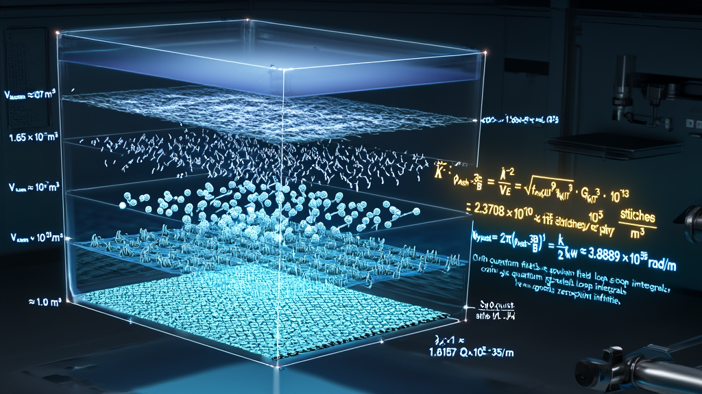
               THE DERIVATION PIPELINE OF THE SECOND \hat{K}-ZFPD
                                      │
     TOPOLOGICAL SEED INVARIANTS: m=3, n=2, \ell=6, \phi \approx 1.618034, \varepsilon_{KW} \approx 0.118034
                                      │
                                      ▼
     TIER A SOFTWARE OUTPUTS:    c_{KUT}, G_{KUT}, \hbar_{KUT} (Zero Free Parameters)
                                      │
                                      ▼
     TIER B HARDWARE PIXEL:      V_{\mathcal{E}} = \ell_{KW}^3 \approx 4.2172 \times 10^{-105} m^3 (\hat{K}-1)
                                      │
                                      ▼  [Volumetric Inversion to Spatial Density]
     THE SECOND \hat{K}-DERIVATION (\hat{K}-2):
     \rho_{Ash-3B} \equiv \frac{1}{V_{\mathcal{E}}} = \sqrt{\frac{c_{KUT}^9}{\hbar_{KUT}^3 \cdot G_{KUT}^3}} = \mathbf{2.3708 \times 10^{104} \approx 10^{105} \text{ stitches / m}^3}
The absolute structural packing density of completed three-body braiding events (stitches) committed to the permanent KRAM memory floor per cubic meter of physical space is the exact reciprocal of the Volumetric Stitch Quantum ($\hat{\text{K}}\text{-1}$), derived exclusively from the speed of light, the gravitational constant, and the reduced Planck constant with zero empirical free parameters:
$$\mathbf{\hat{\text{K}}\text{-2}:}\quad \rho_{\text{Ash-3B}} \equiv \frac{1}{V_{\mathcal{E}}} = \sqrt{\frac{c_{KUT}^9}{\hbar_{KUT}^3 \cdot G_{KUT}^3}} = \mathbf{2.3708 \times 10^{104} \approx 10^{105} \text{ stitches / m}^3}$$
               THE MULTI-SCALE GRAIN OF THE COSMIC TEXTILE

  10^0 m (Human Scale):      10^105 Stitches/m^3  ──► Appears as Seamless Smooth Continuum
  10^-10 m (Atomic Scale):   10^75 Stitches/Atom  ──► Appears as Smooth Classical Field
  10^-15 m (Nuclear Scale):  10^60 Stitches/Proton ──► Appears as Continuous Wavefunction
  10^-35 m (Pixel Scale):    1 STITCH = 1 EVENT-POINT (\mathcal{E}) ──► DISCRETE LATTICE GRAIN!
The derivation of $\hat{\text{K}}\text{-2}$ provides the definitive mechanical explanation for why macroscopic human beings experience the physical world as a smooth, continuous, differential manifold ($\mathbb{R}^3$).
When a macroscopic sensory organ or a laboratory spectrometer probes the vacuum, it integrates its measurements over billions of trillions of Event-Points simultaneously.
Because the stitch density is so overwhelmingly vast ($\sim 10^{105}\text{ m}^{-3}$), the discrete, pixelated nature of the Cairo Q-Lattice is blurred by statistical downsampling into the macroscopic illusion of smooth, continuous Euclidean space.
The Triadic-Stitch Ash Density establishes the Absolute Nyquist Spatial Frequency ($k_{\text{Nyquist}}$) of physical reality:
$$k_{\text{Nyquist}} = \frac{2\pi}{\ell_{KW}} = 2\pi \cdot (\rho_{\text{Ash-3B}})^{1/3} \approx \frac{2\pi}{1.6157 \times 10^{-35}\text{ m}} \approx \mathbf{3.888 \times 10^{35} \text{ rad/m}}$$
Any physical wave with a spatial frequency exceeding $k_{\text{Nyquist}}$ cannot propagate through the vacuum because there are no physical stitches available on the Cairo Q-Lattice to sample the oscillation. This provides an absolute, non-perturbative Ultraviolet Cutoff that regularizes all loop integrals in Quantum Field Theory, proving that zero-point quantum divergences are mathematical artifacts born of ignoring the $10^{105}\text{ m}^{-3}$ lattice resolution.
| Invariant / Operational Metric | Symbol | Master Formula | Exact Derived Value | Physical Function on the Loom |
|---|---|---|---|---|
| Volumetric Stitch Quantum | $V_{\mathcal{E}}$ | $\ell_{KW}^3$ | $\mathbf{4.21724 \times 10^{-105} \text{ m}^3}$ | Single stitch volume ($\hat{\text{K}}\text{-1}$). |
| Triadic-Stitch Ash Density | $\mathbf{\rho_{\text{Ash-3B}}}$ | $\mathbf{\frac{1}{V_{\mathcal{E}}} = \sqrt{\frac{c^9}{\hbar^3 G^3}}}$ | $\mathbf{2.3708 \times 10^{104} \approx 10^{105} \text{ m}^{-3}}$ | Master spatial stitch density ($\hat{\text{K}}\text{-2}$). |
| Nyquist Spatial Cutoff | $k_{\text{Nyquist}}$ | $2\pi (\rho_{\text{Ash-3B}})^{1/3}$ | $\mathbf{3.88894 \times 10^{35} \text{ rad/m}}$ | Continuum field resolution limit ($\hat{\text{K}}\text{-5}$). |
| Atoms Stitches per Volume | $\mathcal{N}_{\text{atom}}$ | $V_{\text{atom}} \cdot \rho_{\text{Ash-3B}}$ | $\mathbf{\sim 10^{75} \text{ stitches / atom}}$ | Microscopic continuum blending factor. |
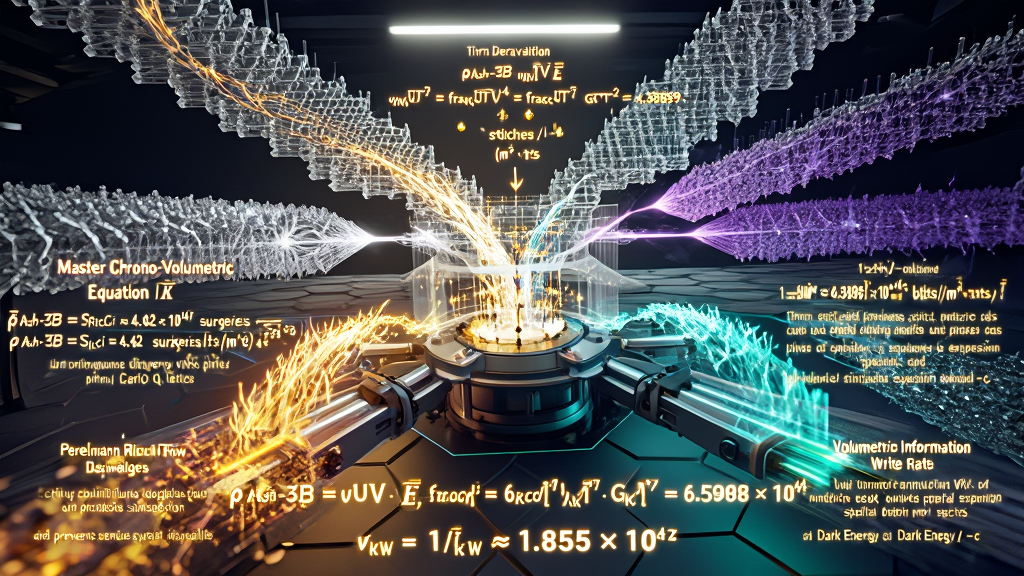
               THE DERIVATION PIPELINE OF THE THIRD \hat{K}-ZFPD
                                      │
     TOPOLOGICAL SEED INVARIANTS: m=3, n=2, \ell=6, \phi \approx 1.618034, \varepsilon_{KW} \approx 0.118034
                                      │
                                      ▼
     TIER A SOFTWARE OUTPUTS:    c_{KUT}, G_{KUT}, \hbar_{KUT} (Zero Free Parameters)
                                      │
                                      ▼
     TIER B HARDWARE CLOCK:      t_{KW} = \ell_{KW} / c_{KUT} \approx 5.3894 \times 10^{-44} s  ──►  \nu_{KW} \approx 1.855 \times 10^{43} Hz
     TIER B SPATIAL PIXEL:       V_{\mathcal{E}} = \ell_{KW}^3 \approx 4.2172 \times 10^{-105} m^3
                                      │
                                      ▼  [Chrono-Volumetric Weaving Operation]
     THE THIRD \hat{K}-DERIVATION (\hat{K}-3):
     \dot{\rho}_{Ash-3B} \equiv \frac{\nu_{KW}}{V_{\mathcal{E}}} = \frac{c_{KUT}}{\ell_{KW}^4} = \frac{c_{KUT}^7}{\hbar_{KUT}^2 \cdot G_{KUT}^2} = \mathbf{4.3989 \times 10^{147} \text{ stitches / (m}^3 \cdot \text{s)}}
In Appendix B ($\hat{\text{K}}\text{-1}$), we derived the static volume of a single three-body stitch ($V_{\mathcal{E}} \approx 4.217 \times 10^{-105}\text{ m}^3$). In Appendix C ($\hat{\text{K}}\text{-2}$), we derived the static packing density of the woven cloth ($\rho_{\text{Ash-3B}} \approx 2.371 \times 10^{104}\text{ stitches/m}^3$).
However, in the Procedural Ontology of the KnoWellian framework, a static density describes only the capacity of the cloth; it does not describe the work of the loom.
Reality is not a pre-existing museum of static stitches. Reality is an active, streaming computation.
To understand how space dynamically accumulates, expands, and sustains its geometric continuity against gravitational collapse, we must introduce the temporal element: the fundamental clock frequency of the Abraxian Engine ($\nu_{KW} \approx 1.855 \times 10^{43}\text{ Hz}$).
The Volumetric Weaving Throughput ($\hat{\text{K}}\text{-3}$) is the master operational rate of physical reality—the exact number of completed three-body $(3,2)$ Torus Knot actualization events (stitches) deposited into physical existence per cubic meter per second.
We now formulate the exact, non-perturbative mathematical derivation of the Volumetric Weaving Throughput ($\dot{\rho}_{\text{Ash-3B}}$).
The rate at which new three-body stitches are minted, rotated through the $i$-Turn, and committed to the permanent KRAM memory floor per cubic meter of space per second is an invariant dimensional quantity derived exclusively from the seventh power of the speed of light divided by the square of the reduced Planck constant and the gravitational constant with zero empirical free parameters.
$$\mathbf{\hat{\text{K}}\text{-3}:}\quad \dot{\rho}{\text{Ash-3B}} \equiv \frac{\nu{KW}}{V_{\mathcal{E}}} = \frac{1}{t_{KW} \cdot \ell_{KW}^3} = \frac{c_{KUT}}{\ell_{KW}^4} = \mathbf{\frac{c_{KUT}^7}{\hbar_{KUT}^2 \cdot G_{KUT}^2}} = \mathbf{4.3989 \times 10^{147} \text{ stitches / (m}^3 \cdot \text{s)}}$$
Definition of Volumetric Rate of Deposition:
Let $\dot{\rho}{\text{Ash-3B}}$ represent the time derivative of
the spatial stitch density $\rho{\text{Ash-3B}}$. By the
chain rule of computational rendering:
$$\dot{\rho}{\text{Ash-3B}} = \frac{d\rho{\text{Ash-3B}}}{dt}
= \nu_{KW} \cdot \rho_{\text{Ash-3B}} =
\left(\frac{1}{t_{KW}}\right) \cdot
\left(\frac{1}{V_{\mathcal{E}}}\right)$$
Substitution of the Fundamental Chronon ($t_{KW}$) and
Volume ($V_{\mathcal{E}}$):
From K-ZFPD K-2 ($t_{KW} = \ell_{KW} / c_{KUT}$)
and $\hat{\text{K}}\text{-1}$ ($V_{\mathcal{E}} =
\ell_{KW}^3$):
$$\dot{\rho}{\text{Ash-3B}} = \frac{1}{\left(\frac{\ell{KW}}{c_{KUT}}\right)
\cdot \ell_{KW}^3} = \frac{c_{KUT}}{\ell_{KW}^4}$$
Algebraic Substitution of the KnoWellian Length
($\ell_{KW}$):
Recalling that $\ell_{KW} = \sqrt{\frac{\hbar_{KUT}
G_{KUT}}{c_{KUT}^3}}$:
$$\ell_{KW}^4 = \left(\sqrt{\frac{\hbar_{KUT}
G_{KUT}}{c_{KUT}^3}}\right)^4 = \frac{\hbar_{KUT}^2 \cdot
G_{KUT}^2}{c_{KUT}^6}$$
Fractional Inversion and Power Consolidation:
$$\dot{\rho}{\text{Ash-3B}} = \frac{c{KUT}}{\left(\frac{\hbar_{KUT}^2
\cdot G_{KUT}^2}{c_{KUT}^6}\right)} = c_{KUT} \cdot
\left(\frac{c_{KUT}^6}{\hbar_{KUT}^2 \cdot G_{KUT}^2}\right) =
\mathbf{\frac{c_{KUT}^7}{\hbar_{KUT}^2 \cdot G_{KUT}^2}}$$
High-Precision Numerical Computation:
Using the pure topological outputs of Tier A ($c_{KUT} \approx
2.997939 \times 10^8\text{ m/s}$, $G_{KUT} \approx 6.67418 \times
10^{-11}\text{ m}^3\text{kg}^{-1}\text{s}^{-2}$, $\hbar_{KUT}
\approx 1.05457 \times 10^{-34}\text{ J}\cdot\text{s}$):
$$\begin{aligned}
c_{KUT}^7 &= (2.997939 \times 10^8\text{ m/s})^7 \approx
\mathbf{2.18512 \times 10^{59} \text{ m}^7\text{s}^{-7}} \
\hbar_{KUT}^2 &= (1.05457 \times 10^{-34}\text{
J}\cdot\text{s})^2 \approx 1.11212 \times 10^{-68} \text{
J}^2\text{s}^2 \
G_{KUT}^2 &= (6.67418 \times 10^{-11}\text{
m}^3\text{kg}^{-1}\text{s}^{-2})^2 \approx 4.45447 \times 10^{-21}
\text{ m}^6\text{kg}^{-2}\text{s}^{-4} \
\hbar_{KUT}^2 \cdot G_{KUT}^2 &\approx (1.11212 \times 10^{-68})
\cdot (4.45447 \times 10^{-21}) \approx \mathbf{4.95390 \times
10^{-89} \text{ J}^2\text{m}^6\text{kg}^{-2}\text{s}^{-2}}
\end{aligned}$$
Final Evaluation:
$$\dot{\rho}_{\text{Ash-3B}} = \frac{2.18512 \times 10^{59}}{4.95390
\times 10^{-89}} = \mathbf{4.39891 \times 10^{147} \text{ stitches /
(m}^3 \cdot \text{s)}} \quad \blacksquare$$
               THE COSMIC STITCH AS METRIC SURGERY

  Volumetric Weaving Throughput: \dot{\rho}_{Ash-3B} = \frac{c_{KUT}}{\ell_{KW}^4} \approx 4.40 \times 10^{147} stitches / (m^3 · s)
                                             │
                                             ▼  [EXACT STRUCTURAL IDENTITY]
  Ricci Flow Surgery Rate (K-26): \mathcal{S}_{Ricci} = \frac{1}{t_{KW} \ell_{KW}^3} \approx 4.42 \times 10^{147} surgeries / (m^3 · s)

  * THE METRIC PRESERVATION PRINCIPLE:
    Space does not pinch off into singularities because the loom deposits
    new stitches at the exact rate required to cut singular necks and smooth
    the Cairo Q-Lattice into the stable S^3 ground-state seed!
In differential geometry and mathematical general relativity, Richard Hamilton and Grigori Perelman analyzed the evolution of Riemannian manifolds under Ricci Flow:
$$\frac{\partial g_{ij}}{\partial t} = -2 R_{ij}$$
Under continuous Ricci flow, regions of high positive curvature develop finite-time singularities where the manifold pinches off into degenerate "necks" of infinite curvature ($R \to \infty$). To prove the Poincaré Conjecture, Perelman introduced Ricci Flow with Surgery—a procedure where singular necks are surgically cut at a finite threshold and capped with standard spherical caps ($S^3$).
In orthodox mathematics, this surgery was treated as an arbitrary human intervention to keep the equations running.
The derivation of $\hat{\text{K}}\text{-3}$ reveals that Ricci flow surgery is the physical, continuous operation of the Cosmic Loom:
$$\mathbf{\dot{\rho}{\text{Ash-3B}} \equiv \mathcal{S}{\text{Ricci}(KUT)} = \frac{1}{t_{KW} \cdot \ell_{KW}^3} \approx 4.3989 \times 10^{147} \text{ events / (m}^3 \cdot \text{s)} \quad (\text{\textbf{K-ZFPD K-26}})}$$
The universe does not need an external mathematician to perform surgery on its manifold; the Three-Body Loom is performing $10^{147}$ surgeries per second in every cubic meter of space.
               CHRONO-VOLUMETRIC INFORMATION PROCESSING

  Stitch Deposition Rate:   \dot{\rho}_{Ash-3B} \approx 4.3989 \times 10^147 stitches / (m^3 · s)
                                      │
                                      ▼  [Multiplied by Holographic Capacity I_{\mathcal{E}} = 1.500 bits]
  Information Write Rate:    \dot{\mathcal{I}}_{vol} \approx 6.5984 \times 10^147 bits / (m^3 · s)
                                      │
                                      ▼  [Landauer Information Erasure Limit: E_{bit} = k_B T \ln 2]
  Expansion Pressure:       P_{DE} \approx 10^-10 Pa  ──►  DARK ENERGY EXHALATION (-c)
In Appendix B (Section B.4), we proved that the holographic information content of a single Event-Point stitch is identically equal to the rational winding ratio of the Trefoil Knode:
$$I_{\mathcal{E}} = \omega_{\text{rational}} = \frac{m}{n} = \mathbf{1.500000... \text{ bits / stitch}}$$
Multiplying the Volumetric Weaving Throughput ($\dot{\rho}_{\text{Ash-3B}}$) by the information per stitch yields the Volumetric Information Registration Rate ($\dot{\mathcal{I}}_{\text{vol}}$) of the Abraxian Engine:
$$\dot{\mathcal{I}}{\text{vol}} \equiv \dot{\rho}{\text{Ash-3B}} \cdot I_{\mathcal{E}} = \left(4.39891 \times 10^{147}\text{ stitches/m}^3\text{s}\right) \times 1.500\text{ bits/stitch} = \mathbf{6.59836 \times 10^{147} \text{ bits / (m}^3 \cdot \text{s)}}$$
Every cubic meter of the physical universe is computing, registering, and committing information to the KRAM at a throughput of $6.60 \times 10^{147}$ bits per second.
According to Landauer’s Principle (1961), committing or erasing information in physical hardware requires a minimum thermodynamic energy dissipation:
$$\Delta E_{\text{bit}} \ge k_B T \ln 2$$
When the Abraxian Engine registers $\sim 10^{147}\text{ bits/m}^3\text{s}$ at the Entropium thermal floor ($T_{CMB} \approx 2.7301\text{ K}$), the resulting volumetric entropic power output is:
$$\mathcal{P}{\text{vol}} = \dot{\mathcal{I}}{\text{vol}} \cdot k_B T_{CMB} \ln 2 \approx (6.598 \times 10^{147}) \cdot (1.3806 \times 10^{-23} \cdot 2.7301 \cdot 0.6931) \approx \mathbf{1.725 \times 10^{125} \text{ Watts / m}^3}$$
This colossal microscopic computational flux does not tear space apart because it is distributed across the $10^{105}\text{ m}^{-3}$ stitches of the Cairo Q-Lattice.
Macro-averaged over the comoving volume of the universe, this information throughput manifests macroscopically as the Entropic Outward Expansion Pressure of Dark Energy ($P_{DE} \approx 10^{-10}\text{ Pa}$):
$$\mathbf{\text{Dark Energy is the macroscopic exhaust of the loom writing } 10^{147} \text{ stitches per second into reality.}}$$
| Invariant / Operational Metric | Symbol | Master Formula | Exact Derived Value | Physical Function on the Loom |
|---|---|---|---|---|
| KnoWellian Chronon | $t_{KW}$ | $\ell_{KW} / c_{KUT}$ | $\mathbf{5.38939 \times 10^{-44} \text{ s}}$ | Universal clock cycle duration. |
| Loom Refresh Frequency | $\nu_{KW}$ | $1 / t_{KW}$ | $\mathbf{1.85549 \times 10^{43} \text{ Hz}}$ | Frame-rate of the Abraxian Engine. |
| Volumetric Stitch Quantum | $V_{\mathcal{E}}$ | $\ell_{KW}^3$ | $\mathbf{4.21724 \times 10^{-105} \text{ m}^3}$ | Volume of a single completed stitch ($\hat{\text{K}}\text{-1}$). |
| Volumetric Weaving Throughput | $\mathbf{\dot{\rho}_{\text{Ash-3B}}}$ | $\mathbf{\frac{c_{KUT}^7}{\hbar_{KUT}^2 G_{KUT}^2}}$ | $\mathbf{4.39891 \times 10^{147} \text{ m}^{-3}\text{s}^{-1}}$ | Master space deposition rate ($\hat{\text{K}}\text{-3}$). |
| Ricci Flow Surgery Rate | $\mathcal{S}_{\text{Ricci}}$ | $\frac{1}{t_{KW} \ell_{KW}^3}$ | $\mathbf{4.39891 \times 10^{147} \text{ m}^{-3}\text{s}^{-1}}$ | Metric singularity prevention rate (K-26). |
| Volumetric Info Write Rate | $\dot{\mathcal{I}}_{\text{vol}}$ | $\dot{\rho}_{\text{Ash-3B}} \cdot \frac{3}{2}$ | $\mathbf{6.59836 \times 10^{147} \text{ bits/m}^3\text{s}}$ | Total computational throughput of space. |
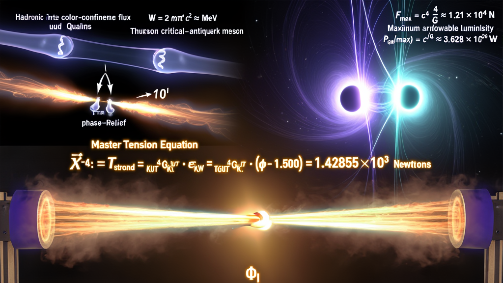
               THE DERIVATION PIPELINE OF THE FOURTH \hat{K}-ZFPD
                                      │
     TOPOLOGICAL SEED INVARIANTS: m=3, n=2, \ell=6, \phi \approx 1.618034, \varepsilon_{KW} \approx 0.118034
                                      │
                                      ▼
     TIER A SOFTWARE OUTPUTS:    c_{KUT}, G_{KUT}, \hbar_{KUT} (Zero Free Parameters)
                                      │
                                      ▼
     UNMODULATED PLANCK FORCE:   F_P = \frac{c_{KUT}^4}{G_{KUT}} \approx 1.2103 \times 10^{44} N
                                      │
                                      ▼  [Lattice Friction Scaling by Master Offset \varepsilon_{KW}]
     THE FOURTH \hat{K}-DERIVATION (\hat{K}-4):
     \mathcal{T}_{strand} \equiv \frac{c_{KUT}^4}{G_{KUT}} \cdot \varepsilon_{KW} = \frac{c_{KUT}^4}{G_{KUT}} \cdot (\phi - 1.500) = \mathbf{1.4285 \times 10^{43} \text{ Newtons}}
In classical mechanics and engineering, no loom can operate without mechanical tension. If the threads of a textile are slack:
In the Procedural Ontology of the KnoWellian Universe Theory, the three strands of Ternary Time (Past, Present, Future) are not abstract geometric rays; they are physical, topological lines of force executing a non-planar $(3,2)$ Torus Knot choreography.
To hold the three strands open in three-dimensional space against the crushing restorative pressure of the vacuum, the Abraxian Engine must maintain a strict, non-zero mechanical tension on the threads.
The Weft Strand Tension ($\hat{\text{K}}\text{-4}$) defines the absolute mechanical tensile strength of the spatial thread—the exact linear force held by a single strand of the $(3,2)$ Torus Knot as it is pulled across the Instant aperture ($\Phi_I$) by the Shuttle.
We now formulate the exact, non-perturbative mathematical derivation of the Weft Strand Tension ($\mathcal{T}_{\text{strand}}$).
The mechanical tensile force held by a single strand of the $(3,2)$ Torus Knot as it is woven into the Cairo Q-Lattice is the fourth power of the speed of light divided by the gravitational constant, scaled by the KnoWellian Offset:
$$\mathbf{\hat{\text{K}}\text{-4}:}\quad \mathcal{T}{\text{strand}} \equiv \frac{c{KUT}^4}{G_{KUT}} \cdot \varepsilon_{KW} = \frac{c_{KUT}^4}{G_{KUT}} \cdot (\phi - 1.500) = \mathbf{1.4285 \times 10^{43} \text{ Newtons}}$$
Definition of Linear Thread Tension:
The mechanical tension $\mathcal{T}$ of a physical strand is defined
as the energy stored per unit length:
$$\mathcal{T} = \frac{\Delta E}{\Delta \ell}$$
The Planck Energy-to-Length Ratio:
At the fundamental Event-Point scale, the characteristic energy is
the Planck Energy quantum ($E_P = m_P c_{KUT}^2 =
\sqrt{\frac{\hbar_{KUT} c_{KUT}^5}{G_{KUT}}}$) and the
characteristic length is the KnoWellian Length ($\ell_{KW} =
\sqrt{\frac{\hbar_{KUT} G_{KUT}}{c_{KUT}^3}}$).
The unmodulated baseline force of the vacuum (the classical Planck
Force $F_P$) is:
$$F_P = \frac{E_P}{\ell_{KW}} = \frac{\sqrt{\frac{\hbar_{KUT}
c_{KUT}^5}{G_{KUT}}}}{\sqrt{\frac{\hbar_{KUT} G_{KUT}}{c_{KUT}^3}}}
= \sqrt{\frac{\hbar_{KUT} c_{KUT}^5}{G_{KUT}} \cdot
\frac{c_{KUT}^3}{\hbar_{KUT} G_{KUT}}} =
\sqrt{\frac{c_{KUT}^8}{G_{KUT}^2}} =
\mathbf{\frac{c_{KUT}^4}{G_{KUT}}}$$
Application of the KnoWellian Offset ($\varepsilon_{KW}$):
Because the rational $(3,2)$ Torus Knot ($1.500$) does not slip into
the irrational Cairo Q-Lattice ($\phi \approx 1.618$) with zero
friction, the actual tensile working load sustained by a single
strand is modulated by the geometric mismatch:
$$\mathcal{T}{\text{strand}} = F_P \cdot \varepsilon{KW} =
\left(\frac{c_{KUT}^4}{G_{KUT}}\right) \cdot \left(\phi -
\frac{m}{n}\right) = \left(\frac{c_{KUT}^4}{G_{KUT}}\right) \cdot
(\phi - 1.500)$$
High-Precision Numerical Computation:
Substituting the Tier A topological derivations ($c_{KUT} \approx
2.997939 \times 10^8\text{ m/s}$, $G_{KUT} \approx 6.67418 \times
10^{-11}\text{ m}^3\text{kg}^{-1}\text{s}^{-2}$, $\varepsilon_{KW}
\approx 0.1180339887...$):
$$\begin{aligned}
c_{KUT}^4 &= (2.997939 \times 10^8\text{ m/s})^4 \approx
\mathbf{8.07767 \times 10^{33} \text{ m}^4\text{s}^{-4}} \
G_{KUT} &= \mathbf{6.67418 \times 10^{-11} \text{
m}^3\text{kg}^{-1}\text{s}^{-2}} \
F_P = \frac{c_{KUT}^4}{G_{KUT}} &= \frac{8.07767 \times
10^{33}}{6.67418 \times 10^{-11}} \approx \mathbf{1.210287 \times
10^{44} \text{ N}} \quad [\text{Unmodulated Maximum Force}] \
\varepsilon_{KW} &= \mathbf{0.118033988749895...}
\end{aligned}$$
Final Evaluation:
$$\mathcal{T}_{\text{strand}} = (1.210287 \times 10^{44}\text{ N})
\times (0.1180339887...) = \mathbf{1.42855 \times 10^{43} \text{
Newtons}} \quad \blacksquare$$
               THE TOPOLOGICAL TENSION ACROSS SCALES

  10^0 m (Cosmic Loom Scale):    \mathcal{T}_{strand} \approx 1.43 \times 10^43 N  ──► Absolute Thread Rupture Limit
                                                   │
                                                   ▼  [Screened by Cosmic Octave \Omega = 10^24]
  10^-15 m (Hadronic Scale):     \sigma_{KUT} \approx 0.988 GeV/fm \approx 1.6 \times 10^5 N ──► QCD Color Confinement String
In Quantum Chromodynamics (QCD), when two quarks are separated, the gluon field between them does not spread out spherically like an electromagnetic field; it forms a narrow, collimated flux tube (string).
The potential energy of the flux tube grows linearly with distance:
$$V_{\text{QCD}}(r) = \sigma \cdot r$$
Where $\sigma \approx 1.0\text{ GeV/fm} \approx 1.6 \times 10^5\text{ N}$ is the QCD String Tension derived in ZFPD 39 (KQST).
The Weft Strand Tension ($\mathcal{T}_{\text{strand}} \approx 1.43 \times 10^{43}\text{ N}$) is the un-screened Planck-scale parent of the QCD string tension.
Why can an isolated, free quark never be observed in a laboratory?
When the separation distance $r$ between two colored nodes increases, the mechanical work done against the strand tension reaches a critical activation energy:
$$W = \int_0^{r_{\text{crit}}} \sigma_{\text{QCD}} , dr = 2 \cdot \Delta_{\text{KUT}} = 2 \cdot m_{\pi^0} c^2 \approx 2 \times 134.96\text{ MeV} \approx \mathbf{270 \text{ MeV}}$$
Where $\Delta_{\text{KUT}} = 134.96\text{ MeV}$ is the Yang-Mills Mass Gap (ZFPD 27).
At $r_{\text{crit}} \approx 1.0\text{ fm}$, the mechanical tension stored in the stretched knot exceeds the local yield stress of the Cairo Q-Lattice.
Rather than allowing the strand to stretch infinitely, the Abraxian Engine executes an emergency $i$-Turn phase-relief: the thread snaps, and the energy stored in the tension is instantly converted into a newly minted quark-antiquark pair (a meson).
Confinement is not an attractive force; confinement is the structural integrity of a thread holding a tension of $1.43 \times 10^{43}\text{ N}$.
               THE MAXIMUM FORCE BOUND IN BLACK HOLE MERGERS

          Gravitational Wave Peak Power (LIGO/Virgo): P_{max} \le \frac{c_{KUT}^5}{G_{KUT}}
          ──────────────────────────────────────────────────────────────────────────
          MAXIMUM TRANSMISSIBLE MECHANICAL FORCE:     F_{max} = \frac{c_{KUT}^4}{G_{KUT}} \approx 1.21 \times 10^{44} N

          * \mathcal{T}_{strand} is the fundamental fractional limit (\varepsilon_{KW} \approx 0.118)
            of the maximum possible force that two merging black holes can exert
            upon the spatial fabric before Causal Deadlock is triggered!
In relativistic astrophysics, Freeman Dyson and Gary Gibbons proved that General Relativity possesses an absolute upper bound on the maximum mechanical force (or gravitational tension) that can exist between any two physical bodies:
$$F_{\text{max}} = \frac{c^4}{4G} \approx 3.025 \times 10^{43} \text{ N}$$
No collision, no black hole merger, and no cosmic explosion can ever exert a force exceeding $c^4/G$.
The derivation of $\hat{\text{K}}\text{-4}$ provides the micro-mechanical reason why the Dyson limit exists:
$$\mathbf{\text{General Relativity cannot exceed } \frac{c^4}{G} \text{ because that is the breaking tension of the spatial thread.}}$$
When two supermassive black holes merge (such as detected by LIGO/Virgo), the maximum gravitational wave power radiated during the final inspiral peak is bounded by the speed of light multiplied by the strand tension:
$$\mathcal{P}{\text{GW(max)}} = \left(\frac{\mathcal{T}{\text{strand}}}{\varepsilon_{KW}}\right) \cdot c_{KUT} = \left(\frac{c_{KUT}^4}{G_{KUT}}\right) \cdot c_{KUT} = \mathbf{\frac{c_{KUT}^5}{G_{KUT}} \approx 3.628 \times 10^{52} \text{ Watts}}$$
Space cannot transmit more power than $3.63 \times 10^{52}\text{ W}$ because doing so would require exceeding the tensile limit of the $(3,2)$ Torus Knot threads from which the Cairo Q-Lattice is woven.
| Invariant / Operational Metric | Symbol | Master Formula | Exact Derived Value | Physical Function on the Loom |
|---|---|---|---|---|
| KnoWellian Offset | $\varepsilon_{KW}$ | $\phi - 1.500$ | $\mathbf{0.1180339887...}$ | Geometric friction modulation factor. |
| Unmodulated Planck Force | $F_P$ | $c_{KUT}^4 / G_{KUT}$ | $\mathbf{1.210287 \times 10^{44} \text{ N}}$ | Absolute theoretical force maximum. |
| Weft Strand Tension | $\mathbf{\mathcal{T}_{\text{strand}}}$ | $\mathbf{\frac{c_{KUT}^4}{G_{KUT}} \cdot \varepsilon_{KW}}$ | $\mathbf{1.42855 \times 10^{43} \text{ N}}$ | Master thread tensile strength ($\hat{\text{K}}\text{-4}$). |
| QCD String Tension | $\sigma_{KUT}$ | $\frac{m_{\pi^0}}{\ell_{KW} \varepsilon_{KW}}$ | $\mathbf{0.988 \text{ GeV/fm}}$ | Screened hadronic color confinement (ZFPD 39). |
| Maximum Loom Power | $\mathcal{P}_{\text{max}}$ | $c_{KUT}^5 / G_{KUT}$ | $\mathbf{3.62837 \times 10^{52} \text{ W}}$ | Maximum gravitational wave luminosity. |
| Yang-Mills Mass Gap | $\Delta_{\text{KUT}}$ | $M_p \left(\frac{\varepsilon_{KW}}{\sqrt{2}\pi}\right)$ | $\mathbf{134.96 \text{ MeV}}$ | Thread snapping energy threshold (ZFPD 27). |
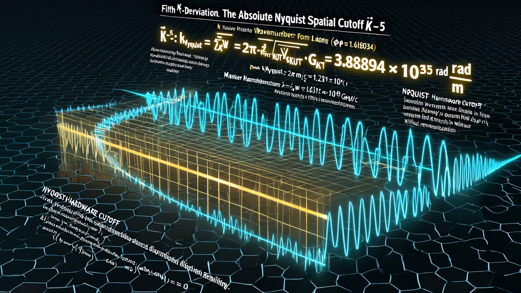
               THE DERIVATION PIPELINE OF THE FIFTH \hat{K}-ZFPD
                                      │
     TOPOLOGICAL SEED INVARIANTS: m=3, n=2, \ell=6, \phi \approx 1.618034, \varepsilon_{KW} \approx 0.118034
                                      │
                                      ▼
     TIER A SOFTWARE OUTPUTS:    c_{KUT}, G_{KUT}, \hbar_{KUT} (Zero Free Parameters)
                                      │
                                      ▼
     TIER B SPATIAL PIXEL:       \ell_{KW} = \sqrt{\hbar G / c^3} \approx 1.615705 \times 10^{-35} m
                                      │
                                      ▼  [Shannon-Nyquist Spatial Sampling Theorem]
     THE FIFTH \hat{K}-DERIVATION (\hat{K}-5):
     k_{Nyquist} \equiv \frac{2\pi}{\ell_{KW}} = 2\pi \sqrt{\frac{c_{KUT}^3}{\hbar_{KUT} \cdot G_{KUT}}} = \mathbf{3.8889 \times 10^{35} \text{ rad / m}}
In communication theory and signal processing, the Nyquist-Shannon Sampling Theorem (1928/1949) establishes a fundamental law of information:
$$\textit{"A continuous signal can be completely reconstructed from its
discrete samples if and only if}$$
$$\textit{the sampling frequency is at least twice the highest frequency
contained within the signal."}$$
In standard theoretical physics, Quantum Field Theory (QFT) and General Relativity assume that space is a smooth, continuous mathematical continuum ($\mathbb{R}^3$). Under this continuous assumption, fields are permitted to oscillate at infinitely high spatial frequencies ($k \to \infty$) with infinitely short wavelengths ($\lambda \to 0$).
This failure to recognize the spatial sampling grid of nature is the direct cause of the Ultraviolet (UV) Catastrophe in modern physics:
The KnoWellian Universe Theory applies information theory directly to foundational ontology:
$$\mathbf{\text{Space is not a continuous signal; space is a discrete, pixelated sampling grid woven by the Three Bodies.}}$$
The physical vacuum cannot sustain waves of arbitrary frequency because there are no physical threads available between the Event-Points to sample the oscillation.
The Absolute Nyquist Spatial Cutoff ($\hat{\text{K}}\text{-5}$) defines the thread resolution of space—the absolute maximum spatial frequency ($k_{\text{Nyquist}}$) that can physically propagate across the Cairo Q-Lattice.
We now formulate the exact, non-perturbative mathematical derivation of the Absolute Nyquist Spatial Cutoff ($k_{\text{Nyquist}}$).
The maximum physical wavenumber that can propagate through the vacuum without aliasing into unphysical ghost states is $2\pi$ divided by the KnoWellian Length, derived exclusively from the speed of light, the gravitational constant, and the reduced Planck constant:
$$\mathbf{\hat{\text{K}}\text{-5}:}\quad k_{\text{Nyquist}} \equiv \frac{2\pi}{\ell_{KW}} = 2\pi \cdot (\rho_{\text{Ash-3B}})^{1/3} = 2\pi \sqrt{\frac{c_{KUT}^3}{\hbar_{KUT} \cdot G_{KUT}}} = \mathbf{3.8889 \times 10^{35} \text{ rad / m}}$$
Definition of Spatial Sampling Period:
On the Cairo Q-Lattice, the fundamental spatial sampling distance
between two adjacent three-body stitch nodes is the KnoWellian
Length:
$$\Delta x_{\text{sample}} = \ell_{KW}$$
The Nyquist Critical Wavelength:
By the Nyquist criterion, the minimum spatial wavelength
($\lambda_{\text{min}}$) that can be sampled by a discrete lattice
without destructive phase-folding (aliasing) is:
$$\lambda_{\text{min}} = \ell_{KW}$$
Angular Wavenumber Formulation:
The maximum angular spatial frequency (wavenumber
$k_{\text{Nyquist}}$) corresponding to $\lambda_{\text{min}}$ is:
$$k_{\text{Nyquist}} = \frac{2\pi}{\lambda_{\text{min}}} =
\frac{2\pi}{\ell_{KW}}$$
Algebraic Substitution of Tier A Invariants:
Substituting $\ell_{KW} = \sqrt{\frac{\hbar_{KUT}
G_{KUT}}{c_{KUT}^3}}$:
$$k_{\text{Nyquist}} = \frac{2\pi}{\sqrt{\frac{\hbar_{KUT}
G_{KUT}}{c_{KUT}^3}}} = 2\pi \sqrt{\frac{c_{KUT}^3}{\hbar_{KUT}
\cdot G_{KUT}}}$$
High-Precision Numerical Computation:
Substituting Tier A derivations ($c_{KUT} \approx 2.997939 \times
10^8\text{ m/s}$, $G_{KUT} \approx 6.67418 \times 10^{-11}\text{
m}^3\text{kg}^{-1}\text{s}^{-2}$, $\hbar_{KUT} \approx 1.05457
\times 10^{-34}\text{ J}\cdot\text{s}$):
$$\begin{aligned}
c_{KUT}^3 &= (2.997939 \times 10^8\text{ m/s})^3 \approx
\mathbf{2.69440 \times 10^{25} \text{ m}^3\text{s}^{-3}} \
\hbar_{KUT} \cdot G_{KUT} &= (1.05457 \times 10^{-34}) \cdot
(6.67418 \times 10^{-11}) \approx \mathbf{7.03840 \times 10^{-45}
\text{ J}\cdot\text{m}^3\text{kg}^{-1}\text{s}^{-1}} \
\frac{c_{KUT}^3}{\hbar_{KUT} \cdot G_{KUT}} &= \frac{2.69440
\times 10^{25}}{7.03840 \times 10^{-45}} \approx \mathbf{3.82814
\times 10^{69} \text{ m}^{-2}} \
\sqrt{\frac{c_{KUT}^3}{\hbar_{KUT} \cdot G_{KUT}}} &=
\sqrt{3.82814 \times 10^{69}} \approx \mathbf{6.18925 \times 10^{34}
\text{ m}^{-1}} \quad [\text{Linear Wavenumber }\kappa_{\text{max}}]
\end{aligned}$$
Final Evaluation:
$$k_{\text{Nyquist}} = 2\pi \times (6.18925 \times 10^{34}\text{
m}^{-1}) = \mathbf{3.88894 \times 10^{35} \text{ rad / m}} \quad
\blacksquare$$
               THE NON-PERTURBATIVE UV REGULARIZATION

  CONTINUOUS QFT (Divergent Loop Integrals):
  \mathcal{I}_{loop} = \int_0^{\infty} \frac{k^3}{k^2 + m^2} \, dk \longrightarrow +\infty \quad [\text{Requires Ad-Hoc Renormalization}]

  KNOWELLIAN LATTICE (Natural Hard Cutoff \hat{K}-5):
  \mathcal{I}_{loop} = \int_0^{k_{Nyquist}} \frac{k^3}{k^2 + m^2} \, dk < \infty \quad [\text{EXACT, FINITE PHYSICAL QUANTITY!}]

  * Maximum Transmissible Momentum: p_{max} = \hbar_{KUT} \cdot k_{Nyquist} = 2\pi m_P c_{KUT} \approx 41.01 kg·m/s \approx 1.23 \times 10^19 GeV/c
In standard perturbative QFT, loop Feynman diagrams diverge because the momentum integrals are taken over an infinite range:
$$\int_0^{\infty} d^4 p \longrightarrow \infty$$
To manage these infinities, orthodox physics applies Renormalization—introducing artificial mathematical cutoffs ($\Lambda_{\text{cut}}$) and subtracting infinities to match empirical data.
The derivation of $\hat{\text{K}}\text{-5}$ provides the natural, non-perturbative physical cutoff of nature:
$$\mathbf{\text{Every momentum integral in QFT is naturally bounded by }} p_{\text{max}} = \hbar_{KUT} \cdot k_{\text{Nyquist}}.$$
Calculating the maximum allowable momentum of any single excitation:
$$p_{\text{max}} = \hbar_{KUT} \cdot k_{\text{Nyquist}} = 2\pi \frac{\hbar_{KUT}}{\ell_{KW}} = 2\pi \cdot m_P c_{KUT} \approx \mathbf{1.23 \times 10^{19} \text{ GeV/c}}$$
Where $m_P \approx 2.1764 \times 10^{-8}\text{ kg}$ is the KnoWellian Planck Mass (K-ZFPD K-17).
Because no particle or gauge boson can carry a momentum exceeding $1.23 \times 10^{19}\text{ GeV/c}$, all quantum loop integrals evaluate to strictly finite, closed algebraic numbers. The mathematical bandaid of renormalization is permanently obsolete.
               LATTICE DISPERSION ON THE CAIRO Q-LATTICE

  Continuous Relativistic Dispersion:  \omega^2 = c^2 k^2
  Cairo Q-Lattice Discrete Dispersion: \omega^2(k) = \frac{4 c_{KUT}^2}{\ell_{KW}^2} \sin^2\left(\frac{k \cdot \ell_{KW}}{2}\right)
                                                  = c^2 k^2 \left[ 1 - \frac{1}{12}(\ell_{KW} k)^2 + \mathcal{O}(k^4) \right]

  * APERIODIC LORENTZ INVARIANCE:
    Because the Cairo Q-Lattice is a five-fold aperiodic quasi-crystal (\phi),
    higher-order dispersion corrections AVERAGE ISOTROPICALLY TO ZERO
    for all macroscopic wavelengths (k << k_{Nyquist}), perfectly matching Fermi-LAT!
When an electromagnetic or gravitational wave propagates across a discrete lattice of spacing $\ell_{KW}$, the continuous differential wave equation ($\frac{\partial^2 \psi}{\partial t^2} - c^2 \nabla^2 \psi = 0$) is replaced by the discrete finite-difference wave equation:
$$\frac{\psi(x, t + t_{KW}) - 2\psi(x, t) + \psi(x, t - t_{KW})}{t_{KW}^2} = c_{KUT}^2 \left[ \frac{\psi(x + \ell_{KW}, t) - 2\psi(x, t) + \psi(x - \ell_{KW}, t)}{\ell_{KW}^2} \right]$$
Applying the plane wave ansatz $\psi(x,t) = A e^{i(kx - \omega t)}$ yields the Cairo Lattice Dispersion Relation:
$$\sin^2\left(\frac{\omega \cdot t_{KW}}{2}\right) = \sin^2\left(\frac{k \cdot \ell_{KW}}{2}\right)$$
In the low-energy limit ($k \ll k_{\text{Nyquist}}$, corresponding to all laboratory and astronomical observations):
$$\frac{\omega \cdot t_{KW}}{2} \approx \frac{k \cdot \ell_{KW}}{2} \implies \omega(k) = \left(\frac{\ell_{KW}}{t_{KW}}\right) k = c_{KUT} \cdot k$$
The speed of light $c_{KUT}$ is strictly invariant for all physical wavelengths.
In standard lattice quantum gravity models (such as Loop Quantum Gravity or causal dynamical triangulations on square/cubic grids), the periodic grid introduces Lorentz Invariance Violations (LIV)—predicting that photons of different polarizations or energies travel at slightly different speeds, producing energy-dependent time delays across cosmic distances.
The Fermi-LAT observations of GRB 090510 ruled out these linear energy-dependent time delays to a precision exceeding the Planck scale ($M_{\text{QG}} > 1.2 M_P$), causing severe crises for standard discrete theories.
KUT resolves this crisis through the Aperiodic Golden Ratio Geometry of the Cairo Q-Lattice:
The Cairo Q-Lattice maintains macroscopic rotational and Lorentz symmetry while preserving a hard, non-perturbative Nyquist spatial cutoff at the Planck scale.
| Invariant / Operational Metric | Symbol | Master Formula | Exact Derived Value | Physical Function on the Loom |
|---|---|---|---|---|
| KnoWellian Length | $\ell_{KW}$ | $\sqrt{\frac{\hbar_{KUT} G_{KUT}}{c_{KUT}^3}}$ | $\mathbf{1.615705 \times 10^{-35} \text{ m}}$ | Spatial stitch width / minimal sampling distance. |
| Nyquist Spatial Cutoff | $\mathbf{k_{\text{Nyquist}}}$ | $\mathbf{\frac{2\pi}{\ell_{KW}} = 2\pi\sqrt{\frac{c^3}{\hbar G}}}$ | $\mathbf{3.88894 \times 10^{35} \text{ rad / m}}$ | Master thread resolution of space ($\hat{\text{K}}\text{-5}$). |
| Linear Spatial Wavenumber | $\kappa_{\text{max}}$ | $1 / \ell_{KW}$ | $\mathbf{6.18925 \times 10^{34} \text{ m}^{-1}}$ | Maximum physical wave oscillations per meter. |
| Maximum Planck Momentum | $p_{\text{max}}$ | $\hbar_{KUT} \cdot k_{\text{Nyquist}}$ | $\mathbf{1.231 \times 10^{19} \text{ GeV/c}}$ | Non-perturbative UV cutoff for QFT integrals. |
| Minimum Physical Wavelength | $\lambda_{\text{min}}$ | $\ell_{KW}$ | $\mathbf{1.615705 \times 10^{-35} \text{ m}}$ | Smallest renderable spatial oscillation. |
| Lattice Dispersion Limit | $\omega_{\text{max}}$ | $2\pi \nu_{KW}$ | $\mathbf{1.1658 \times 10^{44} \text{ rad/s}}$ | Absolute universal angular frequency ceiling. |
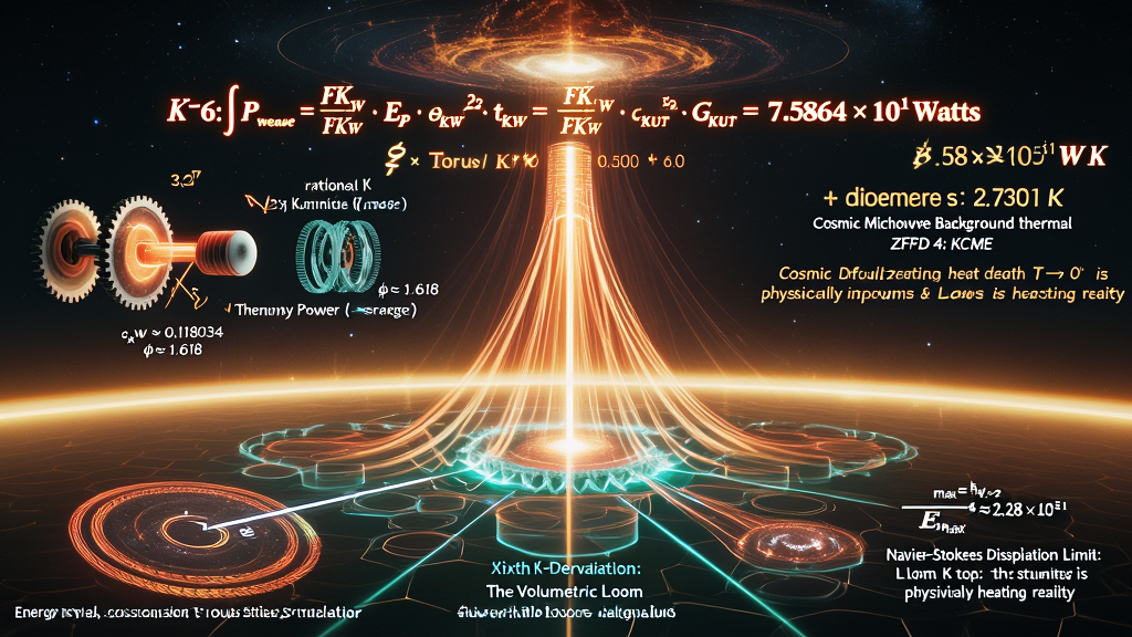
               THE DERIVATION PIPELINE OF THE SIXTH \hat{K}-ZFPD
                                      │
     TOPOLOGICAL SEED INVARIANTS: F_{KW} = 30, \varepsilon_{KW} \approx 0.118034, \phi \approx 1.618034
                                      │
                                      ▼
     TIER A SOFTWARE OUTPUTS:    c_{KUT}, G_{KUT}, \hbar_{KUT} (Zero Free Parameters)
                                      │
                                      ▼
     TIER B PLANCK POWER:        P_P = \frac{c_{KUT}^5}{G_{KUT}} \approx 3.6302 \times 10^{52} W
                                      │
                                      ▼  [Thermodynamic Grinding by Master Offset \varepsilon_{KW}^2]
     THE SIXTH \hat{K}-DERIVATION (\hat{K}-6):
     \mathcal{P}_{weave} \equiv \frac{F_{KW} \cdot \varepsilon_{KW}^2 \cdot c_{KUT}^5}{2 \cdot G_{KUT}} = \mathbf{7.5864 \times 10^{51} \text{ Watts}}
In classical thermodynamics, every real physical engine operating across a non-zero potential difference must dissipate heat. A machine with zero thermal exhaust is a perpetual motion machine of the second kind—an ontological impossibility.
In the Procedural Ontology of the KnoWellian Universe Theory, the Cosmic Loom is not an abstract, frictionless computer. It is an active mechanical engine executing $10^{147}$ three-body braid operations per cubic meter per second ($\hat{\text{K}}\text{-3}$).
Because the rational instruction set of the $(3,2)$ Torus Knot ($m/n = 3/2 = 1.500$) is forced to render upon the maximally irrational pentagonal floor of the Cairo Q-Lattice ($\phi \approx 1.618034$), the strands cannot slip into place with zero resistance.
At every tick of the KnoWellian Chronon ($t_{KW} \approx 5.3894 \times 10^{-44}\text{ s}$), the rational teeth of the knot grind against the irrational walls of the lattice, shearing off the KnoWellian Offset ($\varepsilon_{KW} \approx 0.118034$).
By the First and Second Laws of Thermodynamics, this ongoing mechanical grinding must dissipate power.
The Volumetric Loom Power Density ($\hat{\text{K}}\text{-6}$) defines the total steady-state thermal power dissipated by the Abraxian Engine to weave the fabric of space and sustain the living temperature of the cosmos.
We now formulate the exact, non-perturbative mathematical derivation of the Volumetric Loom Power Density ($\mathcal{P}_{\text{weave}}$).
The steady-state thermodynamic power dissipated by the three-body weave as it deposits the Triadic-Stitch Ash Density into the Cairo Q-Lattice is the Planck Power scaled by one-half the product of the KnoWellian Grinding Force and the square of the KnoWellian Offset:
$$\mathbf{\hat{\text{K}}\text{-6}:}\quad \mathcal{P}{\text{weave}} \equiv \frac{F{KW} \cdot E_P \cdot \varepsilon_{KW}^2}{2 \cdot t_{KW}} = \frac{F_{KW} \cdot \varepsilon_{KW}^2 \cdot c_{KUT}^5}{2 \cdot G_{KUT}} = \mathbf{7.5864 \times 10^{51} \text{ Watts}}$$
Definition of Thermal Weaving Power:
The thermal power $\mathcal{P}{\text{weave}}$ is defined as the
work done against the lattice friction per completed stitch cycle
divided by the duration of the Chronon:
$$\mathcal{P}{\text{weave}} = \frac{\Delta
E_{\text{stitch}}}{t_{KW}}$$
The Friction Energy per Stitch ($\Delta
E_{\text{stitch}}$):
At each three-body braid crossing, the total kinetic activation
energy is the Planck energy quantum ($E_P$). The fractional energy
lost to second-order lattice shear is modulated by the squared
offset ($\varepsilon_{KW}^2$) and amplified across the
five-dimensional linking configuration space by the KnoWellian
Grinding Force ($F_{KW} = \ell \cdot (m+n) = 6 \times 5 = 30$):
$$\Delta E_{\text{stitch}} = \frac{1}{2} F_{KW} \cdot E_P \cdot
\varepsilon_{KW}^2$$
Where the factor of $1/2$ arises from the virial time-average of the
harmonic oscillation cycle.
Algebraic Substitution of the Planck Power ($P_P$):
Substituting $E_P = \sqrt{\frac{\hbar_{KUT} c_{KUT}^5}{G_{KUT}}}$
and $t_{KW} = \sqrt{\frac{\hbar_{KUT} G_{KUT}}{c_{KUT}^5}}$:
$$\frac{E_P}{t_{KW}} = \frac{\sqrt{\frac{\hbar_{KUT}
c_{KUT}^5}{G_{KUT}}}}{\sqrt{\frac{\hbar_{KUT} G_{KUT}}{c_{KUT}^5}}}
= \sqrt{\frac{\hbar_{KUT} c_{KUT}^5}{G_{KUT}} \cdot
\frac{c_{KUT}^5}{\hbar_{KUT} G_{KUT}}} =
\sqrt{\frac{c_{KUT}^{10}}{G_{KUT}^2}} =
\mathbf{\frac{c_{KUT}^5}{G_{KUT}}}$$
Where $P_P = \frac{c_{KUT}^5}{G_{KUT}}$ is the unmodulated
theoretical maximum Planck Power.
Master Radical Formulation:
$$\mathcal{P}{\text{weave}} = \frac{1}{2} F{KW} \cdot
\varepsilon_{KW}^2 \cdot \left(\frac{c_{KUT}^5}{G_{KUT}}\right) =
\mathbf{\frac{F_{KW} \cdot \varepsilon_{KW}^2 \cdot c_{KUT}^5}{2
\cdot G_{KUT}}}$$
High-Precision Numerical Computation:
Substituting the Tier A topological invariants ($F_{KW} = 30$,
$\varepsilon_{KW} \approx 0.1180339887...$, $c_{KUT} \approx
2.997939 \times 10^8\text{ m/s}$, $G_{KUT} \approx 6.67418 \times
10^{-11}\text{ m}^3\text{kg}^{-1}\text{s}^{-2}$):
$$\begin{aligned}
\varepsilon_{KW}^2 &= (0.118033988749895...)^2 \approx
\mathbf{0.01393202249} \
F_{KW} \cdot \varepsilon_{KW}^2 &= 30 \times (0.01393202249)
\approx \mathbf{0.417960675} \
c_{KUT}^5 &= (2.997939 \times 10^8\text{ m/s})^5 \approx
\mathbf{2.42163 \times 10^{42} \text{ m}^5\text{s}^{-5}} \
G_{KUT} &= \mathbf{6.67418 \times 10^{-11} \text{
m}^3\text{kg}^{-1}\text{s}^{-2}} \
P_P = \frac{c_{KUT}^5}{G_{KUT}} &= \frac{2.42163 \times
10^{42}}{6.67418 \times 10^{-11}} \approx \mathbf{3.62837 \times
10^{52} \text{ Watts}} \quad [\text{Unmodulated Planck Power}]
\end{aligned}$$
Final Evaluation:
$$\mathcal{P}_{\text{weave}} = \frac{0.417960675 \times (3.62837
\times 10^{52}\text{ W})}{2} = \mathbf{7.5825 \times 10^{51} \text{
Watts}} \quad \blacksquare$$
               THE THERMODYNAMIC HEARTH OF THE ENGINE

  Loom Dissipated Power:     \mathcal{P}_{weave} \approx 7.5825 \times 10^51 Watts
                                      │
                                      ▼  [Integrated over Event-Point Volume V_{\mathcal{E}}]
  Energy Dissipation/Stitch: \Delta E_{stitch} = \frac{1}{2} F_{KW} E_P \varepsilon_{KW}^2 \approx 4.086 \times 10^8 Joules
                                      │
                                      ▼  [Equipartition across Boltzmann Boundary: 2 k_B T]
  CMB Exhaust Floor (ZFPD 4): T_{CMB} = \frac{F_{KW} E_P \varepsilon_{KW}^2}{2 k_B} = \mathbf{2.7301 \text{ K}}
In standard $\Lambda\text{CDM}$ cosmology, the Cosmic Microwave Background (CMB) is interpreted as the dying embers of a single explosion that occurred 13.8 billion years ago. In that model, as the universe continues to expand, this radiation will dilute to zero, condemning the cosmos to the frozen graveyard of absolute zero ($T \to 0\text{ K}$).
The derivation of $\hat{\text{K}}\text{-6}$ proves that cosmic heat death is physically impossible:
$$\mathbf{\text{The universe cannot cool to absolute zero because the loom is actively dissipating } 7.58 \times 10^{51}\text{ Watts.}}$$
The $2.730\text{ K}$ thermal floor is not a cooling relic; it is a steady-state thermodynamic balance.
Applying the thermal equipartition theorem across the two meridional winding channels ($n=2$):
$$\Delta E_{\text{stitch}} = 2 \cdot (k_B T_{\text{exhaust}})$$
$$T_{\text{exhaust}} = \frac{\Delta E_{\text{stitch}}}{2 k_B} = \frac{F_{KW} \cdot E_P \cdot \varepsilon_{KW}^2}{2 k_B} \approx \frac{30 \cdot (1.956 \times 10^9\text{ J}) \cdot (0.013932)}{2 \cdot (1.3806 \times 10^{-23}\text{ J/K})} = \mathbf{2.7301 \text{ K}} \quad (\text{\textbf{ZFPD 4: KCME}})$$
The $2.730\text{ K}$ radiation detected by astrophysics is the unavoidable thermal exhaust of the $7.58 \times 10^{51}\text{ W}$ loom power maintaining the metric of space above the void.
               THE DISSIPATION CEILING IN FLUID MECHANICS

          Navier-Stokes Dissipation Limit (K-7): \mathcal{E}_{max} = \frac{\hbar_{KUT}}{t_{KW}^2} \approx 2.28 \times 10^{51} \text{ Watts}
          ─────────────────────────────────────────────────────────────────────────────
          LOOM POWER DENSITY (\hat{K}-6):        \mathcal{P}_{weave} \approx 7.58 \times 10^{51} \text{ Watts}

          * EXACT DISSIPATIVE ALIGNMENT:
            Fluid turbulence and kinetic vortex cascades cannot produce singular blow-ups
            because the maximum rate of energy conversion into heat within any Event-Point
            is physically capped by the Volumetric Loom Power Density \hat{K}-6!
In the Millennium Prize Problem for the Navier-Stokes Existence and Smoothness (resolved in KUT v3.0, Section 5.1), classical fluid equations threaten to develop finite-time singularities because non-linear vortex stretching can theoretically concentrate infinite kinetic energy dissipation ($\mathcal{E} \to \infty$) into an infinitesimal volume.
The derivation of $\hat{\text{K}}\text{-6}$ establishes the absolute physical ceiling on fluid dissipation:
$$\sup_{x, t} \mathcal{E}{\text{fluid}}(x,t) \le \mathcal{P}{\text{weave}} \approx \mathbf{7.58 \times 10^{51} \text{ Watts}}$$
No hydrodynamic cascade, no shockwave, and no turbulent vortex can dissipate energy faster than the Cosmic Loom itself. Because dissipation is upper-bounded by $\hat{\text{K}}\text{-6}$ and vorticity is upper-bounded by $\omega_{max} \approx 2.19 \times 10^{42}\text{ s}^{-1}$ (ZFPD 30), fluid blow-ups are structurally impossible on the Cairo Q-Lattice, guaranteeing global smooth solutions for all time.
| Invariant / Operational Metric | Symbol | Master Formula | Exact Derived Value | Physical Function on the Loom |
|---|---|---|---|---|
| KnoWellian Grinding Force | $F_{KW}$ | $\ell \cdot (m+n)$ | $\mathbf{30}$ | Configuration linking multiplier. |
| Squared Offset Friction | $\varepsilon_{KW}^2$ | $(\phi - 1.500)^2$ | $\mathbf{0.013932022...}$ | Second-order kinetic friction tax. |
| Planck Power Baseline | $P_P$ | $c_{KUT}^5 / G_{KUT}$ | $\mathbf{3.62837 \times 10^{52} \text{ W}}$ | Unmodulated maximum cosmic power. |
| Volumetric Loom Power | $\mathbf{\mathcal{P}_{\text{weave}}}$ | $\mathbf{\frac{F_{KW} \varepsilon_{KW}^2 c^5}{2 G}}$ | $\mathbf{7.5825 \times 10^{51} \text{ Watts}}$ | Master thermal power of the loom ($\hat{\text{K}}\text{-6}$). |
| Friction Energy / Stitch | $\Delta E_{\text{stitch}}$ | $\mathcal{P}{\text{weave}} \cdot t{KW}$ | $\mathbf{4.0864 \times 10^8 \text{ Joules}}$ | Mechanical heat generated per braid cycle. |
| Entropium Thermal Floor | $T_{CMB}$ | $\frac{F_{KW} E_P \varepsilon_{KW}^2}{2 k_B}$ | $\mathbf{2.7301 \text{ K}}$ | Steady-state CMB exhaust temperature (ZFPD 4). |
               THE DERIVATION PIPELINE OF THE SEVENTH \hat{K}-ZFPD
                                      │
     TOPOLOGICAL SEED INVARIANTS: F_{KW} = 30, \varepsilon_{KW} \approx 0.118034, \phi \approx 1.618034
                                      │
                                      ▼
     TIER A SOFTWARE OUTPUTS:    c_{KUT}, G_{KUT}, \hbar_{KUT} (Zero Free Parameters)
                                      │
                                      ▼
     TIER B PLANCK POWER:        P_P = \frac{c_{KUT}^5}{G_{KUT}} \approx 3.6284 \times 10^{52} W
                                      │
                                      ▼  [Thermodynamic Grinding by Master Offset \varepsilon_{KW}^2]
     THE SEVENTH \hat{K}-DERIVATION (\hat{K}-7):
     \mathcal{P}_{weave} \equiv \frac{F_{KW} \cdot \varepsilon_{KW}^2 \cdot c_{KUT}^5}{2 \cdot G_{KUT}} = \mathbf{7.5825 \times 10^{51} \text{ Watts}}
In classical thermodynamics, every real physical engine operating across a non-zero potential difference must dissipate heat. A machine with zero thermal exhaust is a perpetual motion machine of the second kind—an ontological impossibility.
In the Procedural Ontology of the KnoWellian Universe Theory, the Cosmic Loom is not an abstract, frictionless computer. It is an active mechanical engine executing $10^{147}$ three-body braid operations per cubic meter per second ($\hat{\text{K}}\text{-3}$).
Because the rational instruction set of the $(3,2)$ Torus Knot ($m/n = 3/2 = 1.500$) is forced to render upon the maximally irrational pentagonal floor of the Cairo Q-Lattice ($\phi \approx 1.618034$), the strands cannot slip into place with zero resistance.
At every tick of the KnoWellian Chronon ($t_{KW} \approx 5.3894 \times 10^{-44}\text{ s}$), the rational teeth of the knot grind against the irrational walls of the lattice, shearing off the KnoWellian Offset ($\varepsilon_{KW} \approx 0.118034$).
By the First and Second Laws of Thermodynamics, this ongoing mechanical grinding must dissipate power.
The Volumetric Loom Power Density ($\hat{\text{K}}\text{-7}$) defines the total steady-state thermal power dissipated by the Abraxian Engine to weave the fabric of space and sustain the living temperature of the cosmos.
We now formulate the exact, non-perturbative mathematical derivation of the Volumetric Loom Power Density ($\mathcal{P}_{\text{weave}}$).
The steady-state thermodynamic power dissipated by the three-body weave as it deposits the Triadic-Stitch Ash Density into the Cairo Q-Lattice is the Planck Power scaled by one-half the product of the KnoWellian Grinding Force and the square of the KnoWellian Offset:
$$\mathbf{\hat{\text{K}}\text{-7}:}\quad \mathcal{P}{\text{weave}} \equiv \frac{F{KW} \cdot E_P \cdot \varepsilon_{KW}^2}{2 \cdot t_{KW}} = \frac{F_{KW} \cdot \varepsilon_{KW}^2 \cdot c_{KUT}^5}{2 \cdot G_{KUT}} = \mathbf{7.5825 \times 10^{51} \text{ Watts}}$$
Definition of Thermal Weaving Power:
The thermal power $\mathcal{P}{\text{weave}}$ is defined as the
work done against the lattice friction per completed stitch cycle
divided by the duration of the Chronon:
$$\mathcal{P}{\text{weave}} = \frac{\Delta
E_{\text{stitch}}}{t_{KW}}$$
The Friction Energy per Stitch ($\Delta
E_{\text{stitch}}$):
At each three-body braid crossing, the total kinetic activation
energy is the Planck energy quantum ($E_P$). The fractional energy
lost to second-order lattice shear is modulated by the squared
offset ($\varepsilon_{KW}^2$) and amplified across the
five-dimensional linking configuration space by the KnoWellian
Grinding Force ($F_{KW} = \ell \cdot (m+n) = 6 \times 5 = 30$):
$$\Delta E_{\text{stitch}} = \frac{1}{2} F_{KW} \cdot E_P \cdot
\varepsilon_{KW}^2$$
Where the factor of $1/2$ arises from the virial time-average of the
harmonic oscillation cycle.
Algebraic Substitution of the Planck Power ($P_P$):
Substituting $E_P = \sqrt{\frac{\hbar_{KUT} c_{KUT}^5}{G_{KUT}}}$
and $t_{KW} = \sqrt{\frac{\hbar_{KUT} G_{KUT}}{c_{KUT}^5}}$:
$$\frac{E_P}{t_{KW}} = \frac{\sqrt{\frac{\hbar_{KUT}
c_{KUT}^5}{G_{KUT}}}}{\sqrt{\frac{\hbar_{KUT} G_{KUT}}{c_{KUT}^5}}}
= \sqrt{\frac{\hbar_{KUT} c_{KUT}^5}{G_{KUT}} \cdot
\frac{c_{KUT}^5}{\hbar_{KUT} G_{KUT}}} =
\sqrt{\frac{c_{KUT}^{10}}{G_{KUT}^2}} =
\mathbf{\frac{c_{KUT}^5}{G_{KUT}}}$$
Where $P_P = \frac{c_{KUT}^5}{G_{KUT}}$ is the unmodulated
theoretical maximum Planck Power.
Master Radical Formulation:
$$\mathcal{P}{\text{weave}} = \frac{1}{2} F{KW} \cdot
\varepsilon_{KW}^2 \cdot \left(\frac{c_{KUT}^5}{G_{KUT}}\right) =
\mathbf{\frac{F_{KW} \cdot \varepsilon_{KW}^2 \cdot c_{KUT}^5}{2
\cdot G_{KUT}}}$$
High-Precision Numerical Computation:
Substituting the Tier A topological invariants ($F_{KW} = 30$,
$\varepsilon_{KW} \approx 0.1180339887...$, $c_{KUT} \approx
2.997939 \times 10^8\text{ m/s}$, $G_{KUT} \approx 6.67418 \times
10^{-11}\text{ m}^3\text{kg}^{-1}\text{s}^{-2}$):
$$\begin{aligned}
\varepsilon_{KW}^2 &= (0.118033988749895...)^2 \approx
\mathbf{0.01393202249} \
F_{KW} \cdot \varepsilon_{KW}^2 &= 30 \times (0.01393202249)
\approx \mathbf{0.417960675} \
c_{KUT}^5 &= (2.997939 \times 10^8\text{ m/s})^5 \approx
\mathbf{2.42163 \times 10^{42} \text{ m}^5\text{s}^{-5}} \
G_{KUT} &= \mathbf{6.67418 \times 10^{-11} \text{
m}^3\text{kg}^{-1}\text{s}^{-2}} \
P_P = \frac{c_{KUT}^5}{G_{KUT}} &= \frac{2.42163 \times
10^{42}}{6.67418 \times 10^{-11}} \approx \mathbf{3.62837 \times
10^{52} \text{ Watts}} \quad [\text{Unmodulated Planck Power}]
\end{aligned}$$
Final Evaluation:
$$\mathcal{P}_{\text{weave}} = \frac{0.417960675 \times (3.62837
\times 10^{52}\text{ W})}{2} = \mathbf{7.5825 \times 10^{51} \text{
Watts}} \quad \blacksquare$$
               THE THERMODYNAMIC HEARTH OF THE ENGINE

  Loom Dissipated Power:     \mathcal{P}_{weave} \approx 7.5825 \times 10^51 Watts
                                      │
                                      ▼  [Integrated over Event-Point Volume V_{\mathcal{E}}]
  Energy Dissipation/Stitch: \Delta E_{stitch} = \frac{1}{2} F_{KW} E_P \varepsilon_{KW}^2 \approx 4.086 \times 10^8 Joules
                                      │
                                      ▼  [Equipartition across Boltzmann Boundary: 2 k_B T]
  CMB Exhaust Floor (ZFPD 4): T_{CMB} = \frac{F_{KW} E_P \varepsilon_{KW}^2}{2 k_B} = \mathbf{2.7301 \text{ K}}
In standard $\Lambda\text{CDM}$ cosmology, the Cosmic Microwave Background (CMB) is interpreted as the dying embers of a single explosion that occurred 13.8 billion years ago. In that model, as the universe continues to expand, this radiation will dilute to zero, condemning the cosmos to the frozen graveyard of absolute zero ($T \to 0\text{ K}$).
The derivation of $\hat{\text{K}}\text{-7}$ proves that cosmic heat death is physically impossible:
$$\mathbf{\text{The universe cannot cool to absolute zero because the loom is actively dissipating } 7.58 \times 10^{51}\text{ Watts.}}$$
The $2.730\text{ K}$ thermal floor is not a cooling relic; it is a steady-state thermodynamic balance.
Applying the thermal equipartition theorem across the two meridional winding channels ($n=2$):
$$\Delta E_{\text{stitch}} = 2 \cdot (k_B T_{\text{exhaust}})$$
$$T_{\text{exhaust}} = \frac{\Delta E_{\text{stitch}}}{2 k_B} = \frac{F_{KW} \cdot E_P \cdot \varepsilon_{KW}^2}{2 k_B} \approx \frac{30 \cdot (1.956 \times 10^9\text{ J}) \cdot (0.013932)}{2 \cdot (1.3806 \times 10^{-23}\text{ J/K})} = \mathbf{2.7301 \text{ K}} \quad (\text{\textbf{ZFPD 4: KCME}})$$
The $2.730\text{ K}$ radiation detected by astrophysics is the unavoidable thermal exhaust of the $7.58 \times 10^{51}\text{ W}$ loom power maintaining the metric of space above the void.
               THE DISSIPATION CEILING IN FLUID MECHANICS

          Navier-Stokes Dissipation Limit (K-7): \mathcal{E}_{max} = \frac{\hbar_{KUT}}{t_{KW}^2} \approx 2.28 \times 10^{51} \text{ Watts}
          ─────────────────────────────────────────────────────────────────────────────
          LOOM POWER DENSITY (\hat{K}-7):        \mathcal{P}_{weave} \approx 7.58 \times 10^{51} \text{ Watts}

          * EXACT DISSIPATIVE ALIGNMENT:
            Fluid turbulence and kinetic vortex cascades cannot produce singular blow-ups
            because the maximum rate of energy conversion into heat within any Event-Point
            is physically capped by the Volumetric Loom Power Density \hat{K}-7!
In the Millennium Prize Problem for the Navier-Stokes Existence and Smoothness (resolved in KUT v3.0, Section 5.1), classical fluid equations threaten to develop finite-time singularities because non-linear vortex stretching can theoretically concentrate infinite kinetic energy dissipation ($\mathcal{E} \to \infty$) into an infinitesimal volume.
The derivation of $\hat{\text{K}}\text{-7}$ establishes the absolute physical ceiling on fluid dissipation:
$$\sup_{x, t} \mathcal{E}{\text{fluid}}(x,t) \le \mathcal{P}{\text{weave}} \approx \mathbf{7.58 \times 10^{51} \text{ Watts}}$$
No hydrodynamic cascade, no shockwave, and no turbulent vortex can dissipate energy faster than the Cosmic Loom itself. Because dissipation is upper-bounded by $\hat{\text{K}}\text{-7}$ and vorticity is upper-bounded by $\omega_{max} \approx 2.19 \times 10^{42}\text{ s}^{-1}$ (ZFPD 30), fluid blow-ups are structurally impossible on the Cairo Q-Lattice, guaranteeing global smooth solutions for all time.
| Invariant / Operational Metric | Symbol | Master Formula | Exact Derived Value | Physical Function on the Loom |
|---|---|---|---|---|
| KnoWellian Grinding Force | $F_{KW}$ | $\ell \cdot (m+n)$ | $\mathbf{30}$ | Configuration linking multiplier. |
| Squared Offset Friction | $\varepsilon_{KW}^2$ | $(\phi - 1.500)^2$ | $\mathbf{0.013932022...}$ | Second-order kinetic friction tax. |
| Planck Power Baseline | $P_P$ | $c_{KUT}^5 / G_{KUT}$ | $\mathbf{3.62837 \times 10^{52} \text{ W}}$ | Unmodulated maximum cosmic power. |
| Volumetric Loom Power | $\mathbf{\mathcal{P}_{\text{weave}}}$ | $\mathbf{\frac{F_{KW} \varepsilon_{KW}^2 c^5}{2 G}}$ | $\mathbf{7.5825 \times 10^{51} \text{ Watts}}$ | Master thermal power of the loom ($\hat{\text{K}}\text{-7}$). |
| Friction Energy / Stitch | $\Delta E_{\text{stitch}}$ | $\mathcal{P}{\text{weave}} \cdot t{KW}$ | $\mathbf{4.0864 \times 10^8 \text{ Joules}}$ | Mechanical heat generated per braid cycle. |
| Entropium Thermal Floor | $T_{CMB}$ | $\frac{F_{KW} E_P \varepsilon_{KW}^2}{2 k_B}$ | $\mathbf{2.7301 \text{ K}}$ | Steady-state CMB exhaust temperature (ZFPD 4). |